Download
1 / 47
470 likes | 699 Vues
Constant Propagation for Loops with Factored Use-Def Chains. Reporter : Lai, Yen-Chang. Outline. Introduction Background Constant Propagation Implementation and Experiment. Introduction.

E N D
Constant Propagation for Loops with Factored Use-Def Chains Reporter:Lai, Yen-Chang
Outline • Introduction • Background • Constant Propagation • Implementation and Experiment
Introduction • Constant propagation analysis is the optimization based on data-flow analysis which is a static (compiler-time) analysis of providing global information about how a procedure manipulates its data. • The solution of constant propagation of one program point is related to the other program points. • Constant propagation is a code reduction technique that determines whether all assignments to a particular variable is a constant and provides the same constant value at certain particular points.
Introduction • A use of the variable at that point can be replaced by the constant. • “Immediate” • Ex. • Result in faster execution than the case that a register must be used to store the constant.
Introduction • The number of times that the loop runs depends on the variables a and b. • Since variables a and b are both constants, the loop iterates constant times.
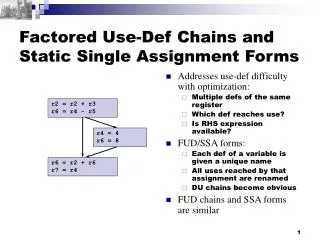
Introduction • A factored use-def (FUD) chain is the SSA (static single assignment) version of the Use-Def chains which readily lend themselves to demand-driven analysis. • Since we want to detect constant values at compile time, it is useful to be able to track constants as they are assigned to variables and then used later.
Introduction(cont.) • A loop is a collection of nodes in a flow graph such that: • All nodes in the collection are strongly connected; that is, from any node in the loop there is a directed path to any other node. • The collection of nodes has a unique entry point, called the ”header”, through which it is the only possible way to reach a node in the loop from a node outside the loop. • There must be at least one way to iterate the loop; ie. there is at least one path that goes back to the header from the nodes in the loop.
Introduction(cont.) • Optimizations often require to collect some information before the loop. • For simplicity of analysis, compilers usually introduce two predecessors to a loop header, namely a preheader and a postbody. • A preheader node is the only one predecessor of the header outside the loop. • The source node of unique back edge is a postbody node.
Introduction(cont.) • Reaching Definition • This determines which definition of a variable may reach each use of the variable in a procedure, and is not killed by another definition. • Dead-Code Elimination • Unreachable codes or their removal does not affect the operations of a program, and hence can be eliminated freely.
Introduction(cont.) • Def-Use link and Use-Def link • A Def-Use link for a variable is a list of all uses that can be reached by a given definition of a variable, while • AUse-Def link is a list of all definitions that can reach a given use.
Background • Control Flow Graph • The statements of a program are grouped into a set of basic blocks. • We write to mean there is a path from X to Y with length greater than zero.(X ≠ Y)
Background(cont.) • Dominate • A node X is said to dominate a node Y in a directed graph if every path from Entry to Y includes X, written as X DOM Y. • If X dominates Y and X≠Y, then X strictly dominates Y, written as X SDOM Y. • Every node n has a unique immediate dominator m such that m≠n, m IDOM n Entry Y ?? X
Background(cont.) • Postdominate • A node w is said to posdominate node v in a directed graph if every path from v to Exit includes w, written as w PDOM v. • If w≠v, then w is said to strictly postdominate v, written as w SPDOM v. v w Exit
Background(cont.) • Control Dependence • Control dependence relations are a more general method to capture the information of essential conditions controlling the execution of code in the program. • A node w is control dependent on edge u → v if u is a decision-point that determines whether w will be executed or not. • That means if control flows from node u to node v along edges u → v, then it will eventually reach node w. u v w z Exit
Background(cont.) • A node w is said to be control dependent on edge (u → v) ∈ E • w postdominates v , and • if w ≠u, then w does not postdominate u. u v w z Exit
Background(cont.) • Static Single Assignment (SSA) • SSA is a representation technique which makes a clear correspondence between the use and the definitions of a variable by giving a unique name. • The two properties of SSA form can be achieved by two key phases knownasФ-placement and renaming. • At the join nodes or merge definitions, there must add a special pseudo form of assignment called a φ-function. • The form of φ-function is
Background(cont.) • In a SSA form, each use is reached by a unique definition, and hence program transformations are simplified. • The code motion of a variable use depends primarily on motion of its unique reaching definition. • Intuitively, the program has been transformed to the representation of flow of values.
Background(cont.) • APT Data Structure • they are join (or merge) points • determine their successor will be executed.
Background(cont.) • For each use, a variable has a unique reaching definition even in a merge conflicting definitions created by control flow, which is represented by a φ-term. • Each use of a variable is marked with a new subscript, while the first one is its label and the others are the definitions that reach this use.
Constant Propagation • ConstantProp – • It is the main procedure that analyzes a procedure starting at the Entry node of the program. • VisitPhi– • It is performed when a normal φ-function is encountered. • The number of times that φ-function is visited is the same as the number of operands within the φ-function. • VisitExp– • It is called to evaluate the effect of each expression. • The two situations that VisitExp is called are: • VisitExp is called once when a flow edge of a node is processed first time • VisitExp is called once each time an incoming SSA edge is processed.
Constant Propagation(cont.) • VisitLoop– • It is called when a loop-header φ is encountered, then visits all operations in the loop. • Check – • It does the recursive call to VisitLoop when a operand is never been visited, and hinges on the computation of Lowlink(X ) to determine whether some node are in the same strongly connected components or not.
Constant Propagation(Cont.) • V is the set of CFG nodes in the program. • Eis the set of CFG edges in the program. • SUCC (v) is the set of successors of CFG node v. • Count(SUCC(v)) is the number of successors of node v. • Target(s) is the use for a Def-Use link s. • Source(s) is the definition of φ-term for a Def-Use link s. • CFGWorkListis a work list of CFG edges, initialized as a list of the successor(s) of the Entry node. • SSAWorkList is a work list of Def-Use links. It is initially empty.
Constant Propagation(Cont.) • ReachableEdge(e) is a flag that determines whether a CFG edge e has been marked as being reachable, or executable; it is initially false for all edges. • ReachableNode(v) for CFG node v is a flag that tells whether the node v is identified as reachable by our algorithm. It is initially false for all node.
Constant Propagation(Cont.) • N is the global counter for assigning preorder numbers, initialized to zero. • LoopStack is a push-down(LIFO) stack of operations, initialized to empty. • NPre(P) is the preorder number assigned to each operation as the al- gorithm builds a depth-first spanning forest, initialized as zero for each operation. • Lowlink(P) keeps track ofwhether each operation has a path to a spanning forest predecessor. • InStack(P) is a flag to keep track of whether each operation is on theWorkList. The flag is initialized as false.
Constant Propagation(cont.) • The techniques of constant propagation support several purposes in optimizing compilers: • Expressions evaluated at compile time need not be evaluated at execution time. • Code that is never executed can be deleted. • Detection of the paths never taken simplifies the control flow of a program. • Since many of the parameters to procedures are constants, using constant propagation with procedure integration can avoid the expansion of code (inline) that often results from native implementations of procedure integration.
Conclusions • The approach preselted here is based ol three fundamental results col- cerlilgcolstaltpropagatiol: • WegmalaldZadeck’s SCC algorithm for conditional constant propagation • Algorithm by Wolfe et al. of finding induction variables • The framework of FUD chains. • Our implementation of constant propagation concentrates on the iterative solver.
Conclusions • To find the constant-valued parameters passed through procedures is a more aggressive of constant propagation analysis. • A destructive solution is treating alyassiglmelt to al array as al assiglmelt of ⊥ regardless of the real content of the array.