Download
1 / 17
480 likes | 2.06k Vues
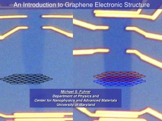
An Introduction to Graphene Electronic Structure. Michael S. Fuhrer Department of Physics and Center for Nanophysics and Advanced Materials University of Maryland. If you re-use any material in this presentation, please credit: Michael S. Fuhrer, University of Maryland. Carbon and Graphene.

E N D
An Introduction to Graphene Electronic Structure Michael S. Fuhrer Department of Physics and Center for Nanophysics and Advanced Materials University of Maryland
If you re-use any material in this presentation, please credit: Michael S. Fuhrer, University of Maryland
Carbon and Graphene - - C - - Carbon Graphene Hexagonal lattice; 1 pz orbital at each site 4 valence electrons 1 pz orbital 3 sp2 orbitals
Graphene Unit Cell Two identical atoms in unit cell: A B Two representations of unit cell: Two atoms 1/3 each of 6 atoms = 2 atoms
Band Structure of Graphene E kx ky Tight-binding model: P. R. Wallace, (1947) (nearest neighbor overlap = γ0)
Band Structure of Graphene – Γ point (k = 0) Bloch states: “anti-bonding” E = +γ0 FA(r), or A B Γ point: k = 0 FB(r), or “bonding” E = -γ0 A B
Band Structure of Graphene – K point FA(r), or FB(r), or K K K λ λ λ K Phase:
Bonding is Frustrated at K point K 0 π/3 5π/3 4π/3 2π/3 π “anti-bonding” E = 0! FA(r), or “bonding” E = 0! FB(r), or K point: Bonding and anti-bonding are degenerate!
Band Structure of Graphene: k·p approximation Hamiltonian: K K’ Eigenvectors: Energy: linear dispersion relation “massless” electrons θkis angle k makes with y-axis b = 1 for electrons, -1 for holes electron has “pseudospin” points parallel (anti-parallel) to momentum
Visualizing the Pseudospin 0 π/3 5π/3 4π/3 2π/3 π
Visualizing the Pseudospin 0 π/3 5π/3 4π/3 2π/3 π 30 degrees 390 degrees
Pseudospin σ || k σ || -k K K’ • Hamiltonian corresponds to spin-1/2 “pseudospin” • Parallel to momentum (K) or anti-parallel to momentum (K’) • Orbits in k-space have Berry’s phase of π
Pseudospin: Absence of Backscattering anti-bonding bonding K’: k||-x K: k||-x K: k||x bonding orbitals anti-bonding orbitals bonding orbitals real-space wavefunctions (color denotes phase) k-space representation K’ K
“Pseudospin”: Berry’s Phase in IQHE holes electrons π Berry’s phase for electron orbits results in ½-integer quantized Hall effect Berry’s phase = π
Graphene: Single layer vs. Bilayer Single Layer vs. Bilayer Single layer Graphene Bilayer Graphene
Graphene Dispersion Relation: “Light-like” Bilayer Dispersion Relation: “Massive” E E ky ky kx kx Massive particles: Light: Electrons in bilayer graphene: Electrons in graphene: Fermi velocity vF instead of c vF = 1x10⁶ m/s ~ c/300 Effective mass m* instead of me m* = 0.033me
Quantum Hall Effect: Single Layer vs. Bilayer Quantum Hall Effect Bilayer: Single layer: Berry’s phase = 2π Berry’s phase = π See also: Zhang et al, 2005, Novoselov et al, 2005.