Understanding Two Models for Air-Water Gas Exchange: a Comparative Analysis
This document comprehensively examines two distinct models of air-water gas exchange: the Two-Film Model and the Surface Renewal Model. It delves into their un-measurable parameters for calculating fluxes, net flux values, and the effects of wind speed on mass transfer coefficients. Key findings highlight how the incorporation of Weibull distribution enhances the accuracy of gas transfer calculations, particularly for CO2, revealing significant underestimations when using mean wind speeds alone. This analysis is crucial for environmental studies involving gas transfer in aquatic systems.

Understanding Two Models for Air-Water Gas Exchange: a Comparative Analysis
E N D
Presentation Transcript
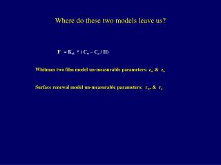
Where do these two models leave us? F = Kol * ( Cw – Ca / H) Whitman two film model un-measurable parameters: zw & za Surface renewal model un-measurable parameters: rw, & ra
Calculation of Flux Net Flux = kol * (Cw – Ca/H*) 1 / kol = 1 / kw + 1 / ka H* Gross fluxes: Volatilization: Water to air transfer Fvolatilization = kol * Cw Absorption: Air to water transfer Fabsorption = kol * Ca/ H* Figure from Schwarzenbach, Gschwend and Imboden, 1993
Processes of Air / Water Exchange “Little” Mixing: Stagnant, 2-film model - “little” wind “More” Mixing: Surface Renewal model – “more” wind Wave Breaking: intense gas transfer ( breaking bubbles) – “even more” wind Figure from Schwarzenbach, Gschwend and Imboden, 1993
Conceptualization of Wind Speed effects on Air/Water Exchange Aerodynamic Transport Region Transfer to broken surface region ~103m Viscous Sublayer ~10-3m Broken Surface Unbroken Surface Figure from Baker, 1996
Effect of Wind Speed on Flux Effect of Wind Speed seen only through changes in Mass Transfer Co-efficient Net Flux = kol * (Cw – Ca/H*) ---- where 1 / kol = 1 / kw + 1 / ka H* Figure from Schwarzenbach, Gschwend and Imboden, 1993
Water Side Mass Transfer Coefficient 1 / kol = 1 / kw + 1 / ka H* Wanninkhof et al. (1991) summarized SF6 experiments in five North American Lakes and found the gas transfer coefficient to be a power function of Wind Speed. The relationship is normalized to the appropriate Schmidt number to relate to the gas transfer of CO2 across the water side boundary layer. kw,CO2 = 0.45 u 1.64 where kw,CO2 is the mass transfer coefficient (cm / hr) across the water layer for CO2 (SC = 600 at 20oC), and u si the wind speed at a 10 m reference height (m/s).
Addition of Weibull distribution in calculation of Kol A two parameter Weibull Distribution can be used to describe the cumulative frequency distribution of wind speeds (Livingstone and Imboden, 1993. Tellus 45B 275-295). F (u) = e ^ –(u / h)x Where F (u) is the probability of a measured wind speed exceeding a given value, u. the form of the distribution curve is determined by the shape parameter, x. The scale of the u-axis is determined by the scale parameter, h . the negative derivative of F(u) yields the corresponding probability density function: f(u) = ( x / u) ( u / h ) x e ^-( u / h ) x Thus, the mean transfer coefficient over the whole range of wind speeds is obtained by integrating the product of the transfer velocity and wind speed probability density f(u). kmean,CO2 = 0 to 8 f(u) *kw(u) * du from Xhang et al. 1999
Weibull distribution - continued Instead of a single mean wind speed value during a sampling period, the wind speed probability density f(u) can be used to account for the effects of a nonlinear wind speed on mass transfer across the water layer over a range of wind speeds during a certain time period. This Weibull distribution can be transformed into a linear form y = ax + b as follows: x = ln u y = ln [ -ln F(u) ] and parameters a & b are determined by linear regression. They are related to the Weibull parameters as follows: x = a h= exp (-b / a) Gas transfer of tracer CO2 can be up to 50% higher when accounting for the non-linear influence of wind speed. Calculations based on mean wind speeds underestimate the total PCB flux to Lake Michigan by as much as 20 to 40% depending upon wind speed variation. from Xhang et al. 1999
Water Side Mass Transfer Coefficient 1 / kol = 1 / kw + 1 / ka H* Wanninkhof et al. (1991) summarized SF6 experiments in five North American Lakes and found the gas transfer coefficient to be a power function of Wind Speed. The relationship is normalized to the appropriate Schmidt number to relate to the gas transfer of CO2 across the water side boundary layer. kw,CO2 = 0.45 u 1.64 where kw,CO2 is the mass transfer coefficient (cm / hr) across the water layer for CO2 (SC = 600 at 20oC), and u si the wind speed at a 10 m reference height (m/s).
Water Side Mass Transfer Coefficient - Continued kw,HOC =kw,mean,CO2 (ScPCB / ScCO2 ) -0.5 = cm s-1 Where Sc is the Schmidt number, the ratio of kinematic viscosity of water and the molecular diffusivity in water. Diffusivity of Hydrophobic organic contaminants (HOCs) through water are calculated using the emperical method of Wilke and Chang (1955). The Schmidt number for CO2 ranges from ~1900 to ~500 for temperatures from 0oC to 25oC according to the equation: ln ScCO2 = -0.052 T +21.71 where ScCO2 is the Schmidt number for CO2 and T is the temperature in K. ScHOC = Ab. Viscosity / (Water Density * Diffusivity of HOC in Water) (g cm-1 sec-1) / ( g cm-3 ) * cm2 sec-1
Water Side Mass Transfer Coefficient - Continued 2 Viscosity, m ( g cm -1 s-1) Density of Water (g cm-1) Diffusivity of PAH in water: Dw,PAHs= 0.0001326/ ((100 * m1.14) * Mol Vol. 0.589) = cm2 sec-1
Air Side Mass Transfer Coefficient – Importance of Density When air temperatures are lower than water temperatures, then air at the water surface is warmer than the ambient air, and thus a density difference exists between the two air layers. The resulting buoyancy can affect the mass transfer at the air/water interface. This influence is not important when average wind speeds are in excess of ~3 m/s at 10 m reference height.
Air Side Mass Transfer Coefficient 1 / kol = 1 / kw + 1 / ka H* Increasing wind speed increases the air-layer mass transfer coefficient approximately linearly: ka,H2O = 0.2 u +0.3 = cm s-1 where ka,H2O is the mass transfer coefficient across the air layer for the tracer H2O (cm / hr) and u is the wind speed. the tracer is related to HOCs through the ratio of air diffusivities (H2O vs. HOC) and can be estimated by the Fuller method: ka,HOC = ka,H2O (DHOC,air / DH2O,air)0.61 where ka,H2O is the mass transfer coefficient (cm / hr) across the air layer for H2O, and u is the wind speed at a 10 m reference height (m/s). Da,PAH = (0.001* (Temp1.75) * ( 1/28.97 + 1/ mol wgt.)0.5) / (20.10.33 + Mol Vol0.33)2 = cm2 s-1 Da,H2O = (0.001* (Temp1.75) * ( 1/28.97 + 1/18)0.5) / (20.10.33 + 180.33)2 = cm2 s-1
Effect of Temperature on Flux Net Flux = kol * (Cw – Ca/H*) ---- ---- 1 / kol = 1 / kw + 1 / kaH* ---- Gross fluxes: Volatilization: Water to air transfer Fvolatilization = kol * Cw Absorption: Air to water transfer Fabsorption = kol * Ca/ H*
Effect of Temperature on Flux – Kol Net Flux = kol * (Cw – Ca/H*) ---- 1 / kol = 1 / kw + 1 / kaH* ----- --- Temperature affects on Kol: Viscosity and Density of water Diffusivity of HOC in water Sc of HOC Sc of CO2 Diffusivity of H20 and HOC in air plus Henry’s law associated effects on Kol (via air side)
Effect of Temperature on Flux – Henry’s Law Net Flux = kol * (Cw – Ca/H*) ---- ---- 1 / kol = 1 / kw + 1 / kaH* ---- Gross fluxes: Volatilization: Water to air transfer Fvolatilization = kol * Cw Absorption: Air to water transfer Fabsorption = kol * Ca/ H*
Indirect Effects of Temperature on A/W Flux Net Flux = kol * (Cw – Ca / H*) ---- Temperature dependence of ambient atmospheric concentrations (and G/P distributions) Gross fluxes: Volatilization: Water to air transfer Fvolatilization = kol * Cw Absorption: Air to water transfer Fabsorption = kol * Ca/ H* log Cair = ao + a1 / T + a2 sin(wd) + a3 cos(wd) after Zhang et al. 1999 Note: possible (and likely) interdependence of T and wind direction
Vapor exchange fluxes and estimated fluxes of HOCs _____________________________________________________________________________ Region Flux (ng/m2 day) Period Reference _____________________________________________________________________________ PCBs Lake Superior +19, +141 August Baker and Eisenreich, 1990 1986 +63 Annual Jeremiason et al., 1994 1992 +13 Annual Jeremiason et al., 1994 +8.3 Annual Hornbuckle et al., 1994 Lake Michigan +8.5-22 Annual Swackhamer and Armstrong,1986 +244 Annual Strachan and Eisenreich,1988 N. Lake Michigan +34 (24-220) Annual Hornbuckle et al., 1995 Lake Ontario +81 Annual Mackay, 1989 Green Bay +13-1300 June-Oct Achman et al., 1993 +111 avg June Achman et al., 1993 Open ocean -40 June-Aug Iwata et al., 1993 +5 Nov-Mar Iwata et al., 1993 Nearshore Chicago -32 to +59 whole year Zhange et al. 1999 northern Chesapeak Bay Nelson et al., 1998 PAHs Baltimore Harbor (1996-1997) Bamford et al., 1999 fluorene +2200 phenanthrene -140 (-140 to 7500) pyrene +590 Southern Chesapeake Bay fluorene +570 February Dickhut and Gustafson, 1995 phenanthrene -570 fluoranthene -140 pyrene -50 Table from Nelson, 1996
Error analysis of Gas exchange calculations Bamford et al. (1999) predicted gas exchange in Baltimore Harbor using Temperature dependent Henry’s Law values, and measured air and water concentrations, along with ambient meteorological parameters (wind speed, water Temperature, etc.). Using estimated uncertainties of 40%, 20%, 20% and 10% for Kol, Cw,Ca, and H resulted in propagated errors of between 43% and 910% of the calculated fluxes. Errors were larger when the fluxes were smallest (i.e. near equilibrium or nearly 0 ng/m2 day net flux), with average error of 64%. Most of the error associated with the fluxes are related to the estimation of Koldue to the effect of wind speed on the kw.