Download
1 / 28
280 likes | 302 Vues
Learn the basics of parallel full matrix algorithms including matrix multiplication and LU decomposition, with applications in computational sciences. Explore matrix and vector operations, solving equations, finding eigenvalues, and more. Dive into examples from chemistry and electromagnetics. Understand broadcast operations, processor groups, and collective communication. Discover Cannon's algorithm for matrix multiplication and performance analysis.

E N D
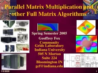
Parallel Matrix Multiplication and other Full Matrix Algorithms Spring Semester 2005 Geoffrey Fox Community Grids Laboratory Indiana University 505 N Morton Suite 224 Bloomington IN gcf@indiana.edu
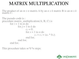
Abstract of Parallel Matrix Module • This module covers basic full matrix parallel algorithms with a discussion of matrix multiplication, LU decomposition with latter covered for banded as well as true full case • Matrix multiplication covers the approach given in “Parallel Programming with MPI" by Pacheco (Section 7.1 and 7.2) as well as Cannon's algorithm. • We review those applications -- especially Computational electromagnetics and Chemistry -- where full matrices are commonly used • Note sparse matrices are used much more than full matrices!
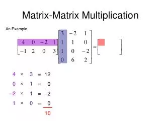
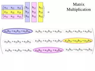
Matrices and Vectors • We have vectors with components xi i=1…n • x = [x1,x2, … x(n-1), xn] • Matrices Aij have n2 elements • A = a11 a12 …a1n a21 a22 …a2n …………... an1 an2 …ann • We can form y = Ax and y is a vector with components like • y1 = a11x1 + a12 x2 + .. + a1nxn .........yn = an1x1 + a12 x2 + .. + annxn
More on Matrices and Vectors • Much effort is spent on solving equations like Ax=b for x x =A-1b • We will discuss matrix multiplication C=AB where C A and B are matrices • Other major activities involve finding eigenvalues λ and eigenvectors x of matrix A Ax = λx • Many if not the majority of scientific problems can be written in matrix notation but the structure of A is very different in each case • In writing Laplace’s equation in matrix form, in two dimensions (N by N grid) one finds N2 by N2 matrices with at most 5 nonzero elements in each row and column • Such matrices are sparse – nearly all elements are zero • IN some scientific fields (using “quantum theory”) one writes Aij as <i|A|j> with a bra <| and ket |> notation
Review of Matrices seen in PDE's • Partial differential equations are written as given below for Poisson’s equation • Laplace’s equation is ρ = 0 • 2Φ= 2Φ/x2 + 2Φ/y2 in two dimensions
Sub-block definition of Matrix Multiply Note indices start at0 for rows and columns of matricesThey start at 1 for rows and columns of processors
The First (“Fox’s” in Pacheco) Algorithm (Broadcast, Multiply, and Roll)
The first stage -- index n=0 in sub-block sum -- of the algorithm on N=16 example
The second stage -- n=1 in sum over subblock indices -- of the algorithm on N=16 example
MPI: Processor Groups and Collective Communication • We need “partial broadcasts” along rows • And rolls (shifts by 1) in columns • Both of these are collective communication • “Row Broadcasts” are broadcasts in special subgroups of processors • Rolls are done as variant of MPI_SENDRECV with “wrapped” boundary conditions • There are also special MPI routines to define the two dimensional mesh of processors
Broadcast in the Full Matrix Case • Matrix Multiplication makes extensive use of broadcast operations as its communication primitives • We can use this application to discuss three approaches to broadcast • Naive • Logarithmic given in Laplace discussion • Pipe • Which have different performance depending on message sizes and hardware architecture
The Pipe Broadcast Operation • In the case that the size of the message is large, other implementation optimizations are possible, since it will be necessary for the broadcast message to be broken into a sequence of smaller messages. • The broadcast can set up a path (or paths) from the source processor that visits every processor in the group. • The message is sent from the source along the path in a pipeline, where each processor receives a block of the message from its predecessor and sends it to its successor. • The performance of this broadcast is then the time to send the message to the processor on the end of the path plus the overhead of starting and finishing the pipeline. • Time = (Message Size + Packet Size (√N – 2))tcomm • For sufficiently large grain size the pipe broadcast is better than the log broadcast • Message latency hurts Pipeline algorithm