Axiomatic semantics
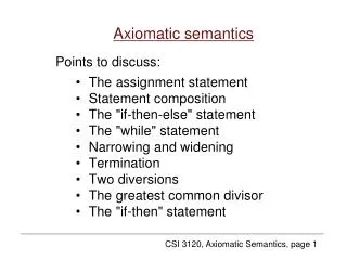
Axiomatic semantics. Points to discuss:. The assignment statement Statement composition The "if-then-else" statement The "while" statement Narrowing and widening Termination Two diversions The greatest common divisor The "if-then" statement. Program verification.

Axiomatic semantics
E N D
Presentation Transcript
Axiomatic semantics Points to discuss: • The assignment statement • Statement composition • The "if-then-else" statement • The "while" statement • Narrowing and widening • Termination • Two diversions • The greatest common divisor • The "if-then" statement
Program verification Program verification includes two steps. • Associate a formula with every meaningful step of the computation. • Show that the final formula logically follows from the initial one through all intermediate steps and formulae.
What is axiomatic semantics? • Axiomatic semantics of assignments, compound statements, conditional statements, and iterative statements has been developed by Professor C. A. R. Hoare. • The elementary building blocks are the formulae for assignments and conditions. • The effects of other statements are described by inference rules that combine formulae for assignments (just as statements themselves are combinations of assignments and conditions).
The assignment statement Let be a logical formula that contains variable v. v e is a formula which we get from when we replace all occurrences of variable v with expression e.
Replacement, an example Before replacement: h>= 0 & h<=n & n > 0 • h 00>= 0 & 0<=n & n > 0 after replacement
Another example m == min( 1 <=i & i <=k–1: ai ) & k–1 <=N kk+1m == min( 1 <=i & i <= (k+1) – 1: ai ) & (k+1)–1 <=N m == min( 1 <= i & i <=k: ai ) & k<=N
The axiom for the assignment statement {ve } v = e {} Example: { 0 >= 0 & 0 <=n & n > 0 } x = 0; { x>= 0 & x<=n & n > 0 }
Two small puzzles { ??? } z = z + 1; { z <= N } { a > b } a = a – b; { ??? }
Statement composition ASSUME THAT {´ } S´ {´´ } and {´´ } S´´ {´´´ } CONCLUDE THAT {´ } S´S´´ {´´´ } In other words: {´ } S´ {´´ } S´´ {´´´ }
A more complicated example x = 0; f = 1; while (x != n) { x = x + 1; f = f * x; } We want to prove that { f == x! }x = x + 1;f = f * x; { f == x! }
The factorial Let's apply the inference rule for composition. ´ is f == x! ´´´ is f == x! S´ is x = x + 1; S´´ is f = f * x;
The factorial (2) We need to find a ´´ for which we can prove: { f == x! } x = x + 1; {´´ } f = f * x; { f == x! } Observe that f == x!f == ((x + 1) – 1)! and therefore f == (x– 1)! xx + 1f == x! That is: { f == x! } x = x + 1;{f == (x– 1)! } ´ ´´ S´
The factorial (3) Now, let us observe that f == (x– 1)! f * x == (x– 1)! * x == x! So, we have f == x! ff * x f == (x– 1)! That is, {f == (x– 1)! }f = f * x;{f == x! } ´´ ´´´ S´´ QED
The "if-else" statement ASSUME THAT {& } S´ {} and { & } S´´ {} CONCLUDE THAT {} if() S ´ else S ´´ {} Both paths through the if-else statement establish the same fact . That is why the whole conditional statement establishes this fact.
"if-else", an example The statement if ( a < 0 ) b = -a; else b = a; makes the formula b == abs(a)true. Specifically, the following fact holds: {true}if ( a < 0 ) b = -a; else b = a;{ b == abs(a) } Here: is true is b == abs(a) is a < 0 Also: S´ is b = -a; S´´ is b = a;
"if-else", an example (2) We will consider cases. First, we assume that is true: true & a < 0a < 0– a == abs(a) Therefore, by the assignment axiom: {– a == abs(a)}b = -a;{b == abs(a)} Similarly, when we assume , we get this: true & a < 0a 0a == abs(a) Therefore: {a == abs(a)}b = a;{b == abs(a)}
"if-else", an example (3) This shows that both S´ and S´´ establish the same condition: b == abs(a) Our fact has been proven: {true}if ( a < 0 ) b = -a; else b = a;{ b == abs(a) } In other words, our conditional statement computes abs(a). It does so without any preconditions: "true" means that there are no restrictions on the initial values of a and b.
The "while" statement A loop invariant is a condition that is true immediately before entering the loop, stays true during its execution, and is still true after the loop has terminated. ASSUME THAT { & } S {} [That is, S preserves .] CONCLUDE THAT { } while ()S { & } providedthat the loop terminates.
The factorial again... x = 0; f = 1; while ( x != n ) { x = x + 1; f = f * x; } Assume that n ≥ 0. After computing x = 0; f = 1; we have f == x! because it is true that 1 == 0!
The factorial again... (2) We showed earlier that { f == x! }x = x + 1; f = f * x;{ f == x! } The reasoning will not change if we add the condition n ≥ 0, because the transitions do not depend on n. So, we can write { n ≥ 0 & f == x! } x = x + 1; f = f * x; { n ≥ 0 & f == x! }
The factorial again... (3) Now, is f == x! is x!=n is x == n Using the inference rule for "while" loops: { n ≥ 0 & f == x! } while ( x != n ) { x = x + 1; f = f * x; } { n ≥ 0 & f == x! & x == n }
The factorial again... (4) Notice that f == x! & x == nf == n! This means two things: { n ≥ 0 } x = 0; f = 1; { n ≥ 0 & f == x! } AND { n ≥ 0 & f == x! } while ( x != n ) { x = x + 1; f = f * x; } { n ≥ 0 & f == n! }
The factorial again... (5) In other words, the program establishes f == n! without any preconditions on the initial values of f and n, assuming that we only deal with n ≥ 0. The axiom for statement composition gives us: { n ≥ 0 } x = 0; f = 1; while ( x != n ) { x = x + 1; f = f * x; } { f == n! } So: this program does compute the factorial of n.
The factorial again... (6) Our reasoning agrees with the intuition of loop invariants: we adjust some variables and make the invariant temporarily false, but we re-establish it by adjusting some other variables. { f == x! }x = x + 1;{ f == (x– 1)! } the invariant is "almost true" { f == (x– 1)! } f = f * x;{ f == x! } the invariant is back to normal This reasoning is not valid for infinite loops:the terminating condition & is never reached, and we know nothing of the situation following the loop.
ASSUME THAT ´ and {} S { } CONCLUDE THAT {´ } S { } ASSUME THAT {} S { } and ´ CONCLUDE THAT { } S { ´ } Narrowing and widening These rules can be used to narrowa precondition, or to widen a postcondition.
Narrowing and widening, a small example n! is computed, for any nonnegative n, with true as the precondition (it is always computed successfully); So, n! will in particular must be computed successfully if initially n == 5.
A larger example (in a more concise notation) { N>= 1 } { N>= 1 & 1 == 1 & a1 == a1 }i = 1; s = a1; { N>= 1 & i == 1 & s == a1 } { N>= 1 & s == a1 + … + ai } INVARIANT while ( i != N ) { { N>= 1 & s == a1 + … + ai & i!= N } i = i + 1; { N>= 1 & s == a1 + … + ai–1 & i – 1 != N } s = s + ai; { N>= 1 & s == a1 + … + ai } } { N>= 1 & s == a1 + … + ai & i == N } { N>= 1 & s == a1 + … + aN }
A larger example (2) • We have shown that this program computes the sum of a1, ..., aN. • The precondition N>= 1 is only necessary to prove termination.
Termination • Proofs like these show only partial correctness. • Everything is fine if the loop stops. • Otherwise we don't know (but the program may be correct for most kinds of data). • A reliable proof must show that all loops in the program are finite. • We can prove termination by showing how each step brings us closer to the final condition.
Once again, the factorial… • Initially, x == 0. • Every step increases x by 1, so we go through the numbers 0, 1, 2, ... • n >= 0 must be found among these numbers. • Notice that this reasoning will not work forn < 0: the program loops.
A decreasing function • A loop terminates when the value of some function of program variables goes down to 0 during the execution of the loop. • For the factorial program, such a function could be n – x. Its value starts at n and decreases by 1 at every step. • For summation, we can take N – i.
Multiplication by successive additions { B>= 0 & B == B & 0 == 0} FOR TERMINATION b = B; p = 0; { b == B & p == 0 }{ p == A * (B–b) } INVARIANT while ( b != 0 ) { p = p + A; { p == A * (B– (b– 1)) } b = b - 1; { p == A * (B–b) } } { p == A * (B–b) & b == 0} { p == A * B } The loop terminates, because the value of the variable b goes down to 0.
Two diversions Prove that the sequence p = a; a = b; b = p; exchanges the values of a and b : { a == A & b == B } p = a; a = b; b = p; { b == A & a == B } The highlights of a proof: { a == A & b == B }p = a; { p == A & b == B }a = b; { p == A & a == B }b = p; { b == A & a == B }
Two diversions (2) Discover and PROVE the behaviour of the following sequence of statements for integer variables x, y: x = x + y; y = x - y; x = x - y;
Two diversions (3) {x == X & y == Y } {x + y == X + Y & y == Y }x = x + y; {x == X + Y & y == Y } {x == X + Y & x - y == X }y = x - y; {x == X + Y & y == X } { x - y == Y & y == X }x = x - y; { x == Y & y == X }
The greatest common divisor { X > 0 & Y > 0 } a = X; b = Y; { } what should the invariant be? while ( a != b ){ & a != b }{ if ( a > b ){ & a != b & a > b } a = a - b; else{ & a != b & (a > b) } b = b - a; } { & (a != b) } { GCD( X, Y ) == a }
GCD (2) We will need only a few properties of greatest common divisors: GCD( n + m, m ) == GCD( n, m ) GCD( n, m + n ) == GCD( n, m ) The first step (very formally): { X > 0 & Y > 0 } { X > 0 & Y > 0 & X == X & Y == Y } a = X; b = Y; { a > 0 & b > 0 & a == X & b == Y }
GCD (3) When the loop stops, we geta == b & GCD( a, b ) == aWe may want this condition in the invariant: a == b & GCD( X, Y ) == GCD( a, b ) At the beginning of the loop, we have: { a > 0 & b > 0 & a == X & b == Y } {a > 0 & b > 0 & GCD( X, Y ) == GCD( a, b ) } So, the invariant could be this: a > 0 & b > 0 & GCD( X, Y ) == GCD( a, b )
GCD (4) We should be able to prove that {a > 0 & b > 0 & GCD(X, Y) == GCD(a, b) & a!=b} while ...... {a > 0 & b > 0 & GCD(X, Y) == GCD(a, b)} The final condition will be a > 0 & b > 0 &GCD(X, Y) == GCD(a, b) & a == b and this will imply GCD( X, Y ) == a
GCD (5) The loop consists of one conditional statement. Our proof will be complete if we show this: {a > 0 & b > 0 & GCD(X, Y) == GCD(a, b) & a!=b} if ( a > b ) a = a - b; else b = b - a; {a > 0 & b > 0 & GCD(X, Y) == GCD(a, b)}
GCD (6) Consider first the case of a > b. {a > 0 & b > 0 &GCD(X, Y) == GCD(a, b) & a!=b & a > b } {a – b > 0 & b > 0 & GCD(X, Y) == GCD(a –b, b)} a = a - b; {a > 0 & b > 0 & GCD(X, Y) == GCD(a, b)}
GCD (7) Now, the case of a > b. {a > 0 & b > 0 & GCD(X, Y) == GCD(a, b) & a!=b & (a > b) } {a > 0 & b–a > 0 & GCD(X, Y) == GCD(a, b–a)} b = b - a; {a > 0 & b > 0 & GCD(X, Y) == GCD(a, b)}
GCD (8) Both branches of if-else give the same final condition. We will complete the correctness proof when we show that the loop terminates. We show how the value of max( a, b ) decreases at each turn of the loop. Let a == A, b == B at the beginning of a step. Assume first that a > b: max( a, b ) == A, so a–b < A,b < A, therefore max( a–b, b ) < A.
GCD (9) Now assume that a < b: max( a, b ) == B, b–a < B, a < B, therefore max( a, b–a ) < B. Since a > 0 and b > 0, max( a, b ) > 0. This means that decreasing the values of a, b cannot go forever. QED
The "if" statement ASSUME THAT { & } S { } and & CONCLUDE THAT { } if ( ) S { }
An example with "if" We will show the following: { N > 0 } k = 1; m = a1; while ( k != N ) { k = k + 1; if ( ak < m ) m = ak; } { m == min( 1 <=i & i <=N: ai ) }
Minimum Loop termination is obvious: the value of N–k goes down to zero. Here is a good invariant: at the kth turn of the loop, when we have already looked at a1, ..., ak, we know thatm == min( 1<=i & i <=k : ai ). Initially, we have this: { N > 0 }k = 1; m = a1; { k == 1 & m == a1 } { k == 1 & m == min( 1<=i & i <=k : ai ) }
Minimum We must prove the following: { m == min( 1<=i & i <=k : ai ) & k!= N } k = k + 1; if ( ak < m ) m = ak; { m == min( 1<=i & i <=k : ai ) }
Minimum (2) { m == min( 1 <=i & i <=k : ai ) & k!=N } { m == min( 1 <=i & i <= (k + 1) – 1: ai ) & (k + 1) – 1 !=N } k = k + 1; { m == min( 1 <=i & i <=k – 1: ai ) & k – 1 !=N } Note that k – 1 !=N ensures the existence of ak.
Minimum (3) This remains to be shown: { m == min( 1 <=i & i <=k – 1: ai ) & k – 1 != N } if ( ak < m ) m = ak; { m == min( 1 <=i & i <=k: ai ) } The fact we will use is this: min( 1 <=i & i <=k: ai ) ==min2( min( 1 <=i & i <=k – 1: ai ), ak )