1 / 0

Supply and Demand Models

Supply and Demand Models. Chapter 3,4. Volatile oil prices . Laws of Supply and Demand. Supply and Demand Framework. A description of a market includes the quantity of goods that are sold in that market, Q , and the price, P , at which they are sold.

hansel
Télécharger la présentation

Supply and Demand Models

An Image/Link below is provided (as is) to download presentation Download Policy: Content on the Website is provided to you AS IS for your information and personal use and may not be sold / licensed / shared on other websites without getting consent from its author. Content is provided to you AS IS for your information and personal use only. Download presentation by click this link. While downloading, if for some reason you are not able to download a presentation, the publisher may have deleted the file from their server. During download, if you can't get a presentation, the file might be deleted by the publisher.

E N D

Presentation Transcript


  1. Supply and Demand Models

    Chapter 3,4
  2. Volatile oil prices
  3. Laws of Supply and Demand
  4. Supply and Demand Framework A description of a market includes the quantity of goods that are sold in that market, Q, and the price, P, at which they are sold. Outcomes in the market are a function of the laws of supply and demand
  5. Law of Demand Ceteris parabis, There is an inverse relationship between the price of a good and the quantity that consumers would like to purchase. What does Ceteris Parabis mean?
  6. Law of Demand Two Explanations: Substitution Effect – Goods purchased to satisfy needs but other goods (substitutes) may also do so. When price rises, consumers have an incentive to switch goods. Income Effect – Consumers have a limited budget. When price of a major item goes up, less money for purchase of all items.
  7. Mathematical representations of Law of Demand Demand Schedule (Spreadsheet) Demand Curve (Geometry) Demand Function (Algebra)
  8. Global Daily Demand Schedule for Oil2010 P = US$ QD = Thousand barrels daily
  9. General Demand Curve P D P2 P1 Q Q2 Q1
  10. Demand Functions An algebraic equation representing demand as a function of the price plus consumer income levels and other factors Example: Linear: QD = a – b × P Exponential: QD = A × P-b
  11. Natural Logarithm Common for professional economists to deal with prices and quantities in natural logarithms z Z z = ln(Z)
  12. Natural Logarithm: p = ln(P) qD = ln(QD) Log-linear Demand qD = a - b × p Natural Logarithm
  13. Law of Supply: Ceteris parabis, there is a positive relationship between the price of a good and the quantity producers bring to the market.
  14. Law of Supply Explanation Increasing Costs Producers will bring goods to market only if the price obtained from selling an extra good will exceed the cost of producing an extra good. If per unit production costs are rising in the number of goods produced, higher prices will be demanded to bring a larger quantity of goods to market.
  15. Mathematical representation of Law of Supply Supply Schedule (Spreadsheet) Supply Curve (Geometry) Supply Function (Algebra)
  16. Global Daily Supply Schedule for Oil2010
  17. Supply Curve S P P2 P1 Q Q1 Q2
  18. Supply Functions An algebraic equation representing supply as a function of the price plus input costs and other factors Examples:
  19. Elasticity as Price Sensitivity
  20. Price Elasticity:The % impact on quantity demanded/suppliedof a 1% change in price
  21. Midpoint Method If you want to calculate a % difference between two points which is the same regardless of which you designate as the reference point (denominator), you can use the average of the two points as the reference point.
  22. Demand Elasticity
  23. A demand curve is classified as INELASTIC if the elasticity is between 0 and 1 Unit elasticity (elasticity equal to 1) is the cutoff point A demand curve is classified as ELASTIC if the elasticity is less than 1
  24. Prices and Revenue Revenue in a market is Revenue = P∙Q If prices change, revenue will change for two reasons: Direct Effect of the Price Change (positive) Indirect Effect of the Price Change on Quantity Demanded (negative) Rule of Thumb: The percentage change in the product of two variables is approximately the sum of the % change in each variable.
  25. Price Elasticity of Revenue If demand is elastic, a price rise reduces revenues If demand is inelastic, a price rise increases revenues
  26. Differences in logarithms approximate midpoint measure of % changes z1 – z0 ≡ ln(Z1) – ln(Z0) ≈ %Z/100
  27. Equilibrium
  28. Equilibrium in the competitive market occurs when the price is set at a level (P*) such that the amount that consumers want to buy is equal to the amount that sellers want to sell (Q*). Excess SupplyIf P were above equilibrium, sellers would want to sell more goods than buyers would want to buy. Competition between sellers would force prices down. Excess DemandIf P were below equilibrium, customers would want to buy more goods than people would want to sell. Competition between buyers would force prices up.
  29. Competitive Market Equilibrium P S D 1 P* Q* Q
  30. Excess Supply at P S D P* Q* Q
  31. Excess Demand at P S D P* Q* Q
  32. Market Equilibrium(Spreadsheet Problem) At what price and quantity (to closest $5) will the oil market clear?
  33. Algebra of Equilibrium QD = a - b×P QS = c + d ×P Linear Functions a - b×P* = c+d×P* (a-c) = (b+d) ×P*
  34. Example
  35. Algebra of Equilibrium qD = a - b×p qS = c + d ×p Log Linear Functions a - b×p* = c+d×p* (a-c) = (b+d) ×p*
  36. Algebra of Equilibrium qD = 11.53 - .05×p qS = 11.14 + .04 ×p Log Linear Functions 11.53 - .05×p* = 11.14+.04×p* (.39) = .09 ×p* 3=11.316
  37. If you know q* and p*, then use antilog function to get Q* and P*
  38. Market Changes:Shifts in Demand & Supply Curves
  39. Shifting Curves/Changing Equilibrium Changes in equilibrium result from shifts in either the demand or supply schedule. We think of shifts in the curves as changes in supply or demand that are caused by factors other than changes in the price of the good. Shifts in the demand curve lead to movements along the supply curve resulting in changes in prices and quantities that move in the same direction. Shifts in the supply curve lead to movements along the demand curve resulting in changes in prices and quantities that move in different directions.
  40. A Shift in the Demand Curve: A parallel increase in the demand schedule at every price point.Price and Quantity Demanded move in same direction P S Shift in the demand curve P** D′ P* D Q* Q** Q
  41. A Shift in the Supply Curve is a Movement along the Demand curve- Price and Quantity Supplied Move in opposite Directions P S′ S D P** P* Q** Q* Q
  42. Equilibrium Effects Price system means that shifts in demand will cause accommodating changes in quantity supplied but also an attenuating change in quantity demanded. Shifts in supply will cause accommodating changes in quantity demanded but also attenuating change in quantity supplied.
  43. A Shift in the Demand Curve: Equilibrium Effect: Movement along the supply curve increases quantity supplied; movement along demand curve ameliorates quantity demanded. S P Along demand curve Along supply curve P** P* D′ D Q* Q** Q
  44. A Shift in the Supply Curve: Equilibrium Effect: Movement along the demand curve reduces quantity demanded; movement along supply curve ameliorates quantity supplied. D S P S′ Along supply curve P** Along demand curve P* Q** Q* Q
  45. Chap. 3, 4 Commodity Markets
  46. Oil Prices Link Why are commodity prices so volatile?
  47. Price Sensitivity and Equilibrium Effects When supply or demand curves shift, the effect will be felt in some combination of changes in prices and quantities. The degree to which changes in either supply or demand are felt in quantity changes rather than price changes is determined by price sensitivity of both demand and supply.
  48. . Steeper (less price sensitive) supply curve means that a demand shift will have a smaller impact on quantity and bigger impact on price. S1 P S2 1 P1** 2 P2** 0 P* D’ D Q Q* Q1** Q2**
  49. . Steeper (less elastic) demand curve means that a supply shift will have a smaller impact on quantity and bigger impact on price. S’ P S 1 P1** 2 P2** 0 P* D2 D1 Q Q2** Q* Q1**
  50. Algebra of Equilibrium Effects If demand or supply elasticitiesare big, effects of supply or demand change on equilibrium price will be small
  51. What determines price elasticity? Availability of Substitutes A price increase will lead to a shift away from the use of a product and toward other products. Price elasticity will be stronger if there are readily available substitutes for a good. A price increase for one good reduce income available for purchases for all goods Price elasticity will be stronger if a good makes up a big chunk of income. World Bank Tobacco Download
  52. Commodities have very inelastic demand. Estimate of elasticity of demand for oil in the US is .061 J.C.B. Cooper, OPEC Review, 2003) Comparisons of Demand Price Elasticities Price Elasticities of Other Goods
  53. Elasticities Extreme P Perfectly Inelastic Demand (Insulin) D Perfectly Elastic Demand (Clear Pepsi) D Q
  54. Elasticity of Supply Elasticity of supply curve depends on the ability of production sector to ramp up supply without increasing the marginal cost of production. A good that is produced with readily available factors w/o a need for time consuming investment will have an elastic supply curve.
  55. Elasticities: Supply Perfectly Inelastic Supply (Van Gogh Paintings) P Perfectly Elastic Supply (Foot Massage) S S Q
  56. Price Elasticity and Time
  57. Elasticity of Demand Short-term vs. Long-term It takes time to find substitutes for goods or to adjust consumption behavior in response to a change in prices. The long-run demand response to a price rise is larger than the short-run. Price elasticity of demand is more negative in the long run than in the short run. .
  58. Oil Demand much more elastic in long run than short-run (J.C.B. Cooper, OPEC Review, 2003)
  59. Price Elasticity of Supply Firms also find it easier to adjust production in the long-run than the short run. Long-run price elasticity of supply is typically greater than short-run OECD study suggests price elasticity of oil supply is .04 in short run and .35 in long run.
  60. Demand Curves
  61. Oil Supply Curves
  62. Income Elasticity/ Cross Price Elasticity Changing Equilibrium
  63. What shifts a demand curve? Changes in consumer preferences Changes in (current or future) consumer income Changes in the prices of other goods that are complementary to or substitutes for other goods. Changes in expected future prices.
  64. Income Elasticity We measure the effect of income on demand for a good as % effect on demand of a 1% increase in income. For normal goods, income elasticity is positive. For inferior goods income elasticity is negative.
  65. Luxuries vs. Necessities There are two types of normal goods. Luxuries take up an increasing share of income as your income grows. Luxuries are income elastic - the income elasticity of luxuries is greater than 1. Necessities take up a declining share of income as your income grows. Necessities are income inelastic – the income elasticity of luxuries is less than 1. China’s Emerging Middle Class Download
  66. Inferior Goods Range of Income Elasticities Normal Goods 1 0 Income Elastic (Luxury Goods) Income Inelastic (Necessities)
  67. Source: OECD study Income Elasticity of Oil Assume a world income elasticity of .5 and an increase of world income equal to 5%. Demand shifts out by 2.5%. Would oil production supplied increase by 2.5%?
  68. Market Equilibrium(Spreadsheet Problem) At what price and quantity (to closest $5) will the oil market clear?
  69. Algebra of Equilibrium Effects 2.5% Shift in Demand Curve
  70. Expected Income Effect Households are forward looking. If they expect income in the future they will increase spending today. Optimism (or pessimism) about future income will shift demand curve.
  71. Changes in Prices of Other Goods For any good there are two types of other goods which are relevant to its demand Substitutes: Those other goods which can take the place of the good of interest (bacon vs. ham) Complements: Those other goods whose use will enhance the value of the good of interest. (bacon and eggs) What are substitutes and complements for oil
  72. Substitutes vs. Complements A good is defined as a “Substitute” when a rise in its price leads to a shift out/up in the demand curve for the good of interest. A good is defined as a “Complement” when a rise in its price leads to a shift in/down in the demand curve for the good of interest.
  73. Cross Price Elasticity Cross price elasticity is the % effect on the quantity demanded of a % change in another price. Goods with positive cross-price elasticities are called substitutes Goods with negative cross-price elasticities are called complements 0 Complements Substitutes
  74. What Shifts the Supply Curve Supply curves represent the extra cost of producing a good which increases in the number of goods produced. But other factors may affect cost besides scale. Cost Shifters Changes in prices of factors of production Changes in prices of related goods Changes in Technology State of Nature Changes in Taxes on Producers Market entry
  75. Speculation & Supply Some commodities have a time dimension. Producers have a choice about when to bring goods to market. If producers believe prices will be higher in the future, they have an incentive to delay shipment to the future. Higher price expectations will shift the supply curve inward. Note: This won’t work for apples, oranges or other perishable commodities.
  76. Expectations of Increased Prices in the Future Lead to Higher Prices Today! P S′ S D P** P* Q** Q* Q
  77. Speculation & Demand For some storable commodities (e.g. gold) or durable goods, expectations of future price hikes might also lead consumers to start buying immediately. Higher price expectations will shift demand curve outward.
  78. Even higher prices! P D' S' S D P*** P** P* Q** Q* Q
  79. Bubbles If current prices can be driven by expectations of even higher prices in the future…and…investors pile into commodities whose price has risen, then this could generate a feedback loop featuring rapidly rising prices Think about for fun. Too theoretical for exam.
  80. Learning Outcomes Solve for equilibrium price and quantities using graphical supply and demand model or spreadsheet supply and demand schedules or simple linear algebra. Explain qualitatively and calculate quantitatively, the likely consequences for equilibrium prices and quantities resulting from exogenous shifts in supply and demand. Calculate elasticities using the midpoint method.
  81. Learning Outcomes Distinguish substitutes/complements, luxuries/necessities/inferior goods. Identify the impact of demand & supply elasticity on price and quantity volatility in the short and long run. Identify the impact of expectations of the future on current prices.
More Related