Download
1 / 20
200 likes | 382 Vues
SERENA Meeting. THE EXOSPHERE OF MERCURY: SODIUM OBSERVATIONS AND MAGNETOSPHERIC MODELLING. Mikonos 2009. Valeria Mangano & Stefano Massetti Interplanetary Space Physics Institute (IFSI) Roma, Italy. TNG ( June 2005). Alt-Az telescope Primary Mirror 3.58 m SARG

E N D
SERENA Meeting THE EXOSPHERE OF MERCURY:SODIUM OBSERVATIONS AND MAGNETOSPHERIC MODELLING Mikonos 2009 Valeria Mangano & Stefano Massetti Interplanetary Space Physics Institute (IFSI) Roma, Italy
TNG (June 2005) Alt-Aztelescope PrimaryMirror 3.58 m SARG Echellespectrograph Nasmythtelescope focus B Resolution: 46000-164000 (in our case 115000) Nafilter 60 Ǻ (no orderoverlapping) Long slit (26.7” x 0.4”) CCD dimension 2 K x 4 K pixels Altitude 2387 m a.s.l. Lat. 28º 45’ 28” N Long. 17º 53’ 38” W Telescopio Nazionale Galileo Roque de Los Muchachos, La Palma
Observationsperformedbetween 29th June and 1st July, at sunset (about 19:00 UT, 1 h) Sun-MercuryDistance 0.422-0.423 AU Illuminatedfraction 57 -54 % AngularDiameter 6.7-7.0 ” ApparentMagnitude 0.05-0.15 Elongation (East) 24.2-24.9º TrueAnomaly Angle 124-130º Sun-Mercury-Earthphase angle 81-85º Exposuretime: 120” Scan in the N-S direction: equator± 6”
Pre-Analysis • Cut + bias and flat-field corrections • Straightening + Calibration D2 (D.shifted from 5895.92 Ǻ) D2 D1 D1 (D.shifted from 5889.92 Ǻ) Sodium of the SOLAR ATMOSPHERE: ABSORPTION (shifted of the sum of Mercury-Earth BANDS and Sun-Mercury relative velocities) Sodium in the EXOSPHERE of MERCURY:EMISSION (shifted by the Mercury-Earth rel. velocity) LINE
Analysis/1 • Correcting spectra for diffuse light 2. Looking for the best profile to fit the Fraunhofer absorptions and further extract the emission lines
Analysis/2 3. Creation of a surface reflectance model devoted to reproduce the soil emission (following the Hapke theory) 4. Comparison of the Hapke model with the observed continuum to derive the conversion: ADU kiloRayleigh Finally, spatial plots of the D1 and D2 lines are deduced.
Results June 29th, 2005 • Twomainfeatures: • Higherintensitiesduring the second night • Southernhemispherepeak June 30th, 2005 July 1st, 2005
coronal hole SoHO/EIT (Fe XV 284 Å) image Interpretation/1(Possible related solar events) Active Region AR0781 CMEs) • Coronal hole on the Sun and an associated high speed stream: • Three different CMEs from the active region AR0781 occurred during the observations: • stream at 650-700 km/s • arrived at Mercury 2-3 days before • carried with it an IMF Bx > 0 for several days SOHO/LASCO CME catalog(http://cdaw.gsfc.nasa.gov/CME_list/)
CME 1: (Halo CME) • 28th June halo CME 16:30 UT, observed initial speed V0 = 1750 km/s. • It was estimates that the CME decelerated from 1750 to 400km/s, in about 6h (~0.144 AU), then it reached Mercury at 0.42 AU after about 30h (hence: 30th June 2005, at about 05:00 UT). • CME 2: • 28th June 20:06 UT, PA = 97˚, AW = 68˚, V(?) 600 km/s • Estimated arrival time @0.42 AU: • 30-June, 03:00 UT (assuming the speed of 600 km/s) • 30-June, 15:00 UT (assuming the speed of 400 km/s) • CME 3: • 29th June 07:31 UT , PA = 83˚, AW = 49˚,V(?) 350 km/s • Estimated arrival time @0.42 AU: 01-July, 17:00 UT
Time sequence of the events CME#1 CME#3 29-Jun (180) 30-Jun (181) 01-Jul (182) 20:00 UT 20:00 UT 20:00 UT time IMF Bx < 0 CME#2 Fast Stream (176)
Interpretation/2(Possible relation with the surface) • Peak coordinates: 250-290º E, 10-40º S • Radar bright spots: (A. Sprague) A (15° E, 25° S), B(15° E, 55° N),C(120° E,15°N) • (J. Harmon) A (12° E, 34° S), B(17° E, 58° N),C(114° E, 11°N), • (18° E, 27° S), Bartok crater No corrispondence can be found!
Interpretation/3(Southern Hemisphere peak) The ion sputtering process (or chemical sputtering + PSD!) caused by plasma precipitation from the magnetosheath through the dayside cusp regions, is highly affected by both the orientation of the Interplanetary Magnetic Field and the solar wind dynamic pressure. In particular, high hemispherical asymmetries are expected because of the dominating radial IMF component at Mercury. June 30th, 2005 PROBLEM: the knowledge of the IMF orientation at the orbit of Mercury is needed to compute the magnetospheric configuration (true both for ground- and space-based observations)
An indirect estimation of the IMF direction at Mercury can be achieved on the basis of the measured solar magnetic field … Wilcox Solar Obs. photospheric field CR#2031
The coronal magnetic field is calculated from photospheric field observations with a potential field model. The field is forced to be radial at the source surface to approximate the effect of the accelerating solar wind on the field configuration (-) → IMF < 0 (+) → IMF > 0
Taking into account the propagation times (3-5 days), we can find the relationship between the coronal magnetic sectors (WSO, ground obs.) and the sign of the IMF radial component at Earth (ACE, L1), and then try to estimate the most likely IMF orientation at Mercury 188 184 180 176 172 IMF Bx (GSE) ? time (-) → IMF < 0 → IMF Bx (GSE) > 0 (+) → IMF > 0 → IMF Bx (GSE) < 0
A more consistent estimation can be derived by means of 3-D numerical simulations of the solar wind/IMF propagation into the heliosphere: 1) Hakamada-Akasofu-Fry (HAF) kinematic solar wind model (gse.gi.alaska.edu) 2) ENLIL magnetohydrodynamic helispheric model (ccmc.gsfc.nasa.gov) - - + Mercury + - - (adapted from original)
Simulations diverge progressively as the distance from the source surface (Sun) increases, but are in relatively good agreement at the orbit of Mercury In the time-period 29th June - 1st July there were 3 or 4 IMF magnetic sectors (depending on the simulation) with Mercury very likely embedded in a negative IMF (i.e. toward the Sun) In the planet’s MSO reference frame (Mercury-Solar-Orbital) a negative IMF means a positive IMF Bx component, which imply a direct IMF reconnection, hence, preferred H+ precipitation in the southern hemisphere … - + Mercury - H+ flux (cm-2 s-1)
Tail Analysis • Potter et al., 2002: • June 5th 2000 TAA= 114º • May 26th 2001 TAA= 125º • Our data: • June 29th 2005 • July 1st 2005 TAA= 124-130º
All dates display similar shape similarTAAs • Dependance more on TAA values than on ejecting phenomena (SW)
Conclusions • Sodium observations campaign are performed at both TNG (2002/03/05/06/09) and THEMIS (2007/08/09… full-disk) observatories, and since June 2006 are part of an international observational campaign in preparation of the BepiColombo mission. • Observations precision need to be improved -> full-disk (THEMIS obs.) • Coordinated Earth-based observations are needed to cross-check the measurements, in particular longer runs are needed to better study the hermean environment and quantify the contribution to the exosphere of the different processes. • They evidenced definite features and suggest a relationship with the Solar Events and/or with the Interplanetary Magnetic Field. • Heliospheric IMF/SW numerical simulations are needed to analyze ground- and space-based data from the magnetospheric point of view. • Paper just published on ICARUS (Mangano et al. 2009)