Download
1 / 24
240 likes | 395 Vues
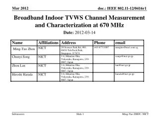
Broadband Indoor TVWS Channel Measurement and Characterization at 670 MHz. Date: 2012-03-14. Abstract. An introduction to indoor TVWS channel measurement and results at 670 MHz. Measurement Setup and Calibration. Measurement targets: Multipath delay spread, particularly, RMS delay spread

E N D
Ming-Tuo ZHOU, NICT Broadband Indoor TVWS Channel Measurement and Characterization at 670 MHz • Date: 2012-03-14
Ming-Tuo ZHOU, NICT Abstract • An introduction to indoor TVWS channel measurement and results at 670 MHz
Ming-Tuo ZHOU, NICT Measurement Setup and Calibration • Measurement targets: • Multipath delay spread, particularly, RMS delay spread • Channel impulse response • Path loss properties • Signaling: • BPSK signal, 20 Mbps, 511-length pseudo random (PN) sequence, central frequency at 670 MHz • CW signal, central frequency at 670 MHz, for path loss measurement • Method: • Custom designed receiver captures transmitted BPSK signal for measurement of multipath delay spread and channel impulse response • For path loss measurement, the received signal power is measured by using a R&S FSU spectrum analyzer
Ming-Tuo ZHOU, NICT Measurement Setup and Calibration -- Instruments Used • Transmitter • Receiver & Spectrum Analyzer
Ming-Tuo ZHOU, NICT Calibration Setup
Ming-Tuo ZHOU, NICT Measurement setup
Ming-Tuo ZHOU, NICT Measurement Parameters
Ming-Tuo ZHOU, NICT Measurement Scenarios 1 – Office 1 – small size office/lab • 185 sqm (=14.52 m×12.74 m) • Includes staff room, 3 experiment rooms, director room, meeting room, kitchen, reception, etc • Walls material: plywood/concrete • Three transmitter antenna locations • Tx antenna – 2.3m, Rx antenna – 0.7m
Ming-Tuo ZHOU, NICT Measurement Scenarios 2 – Office 2 – medium size office/lab • Includes two hall rooms, a conference room, several experiment rooms, a big lab room, store room, staff cubicle area • Walls material: plywood/concrete • One transmitter antenna position • Tx antenna – 2.6m, Rx antenna – 1.4m
Ming-Tuo ZHOU, NICT Some Pictures of Measurement Scenarios Office 1, staff room Office 1, meeting room Office 2, office with staff cubicles Office 2, Hall room 1
Ming-Tuo ZHOU, NICT Extracting Rays • For each receiver location, BPSK signal is received and the normalized power delay profile is plot as function of time stamp • A peak detection method is used to extract rays. • First, the calibrated Nyquist pulse is normalized to the peak of received signal power delay profile, and then it is subtracted from the power delay profile • Second, the calibrated Nyquist pulse is normalized to the peak of the remain part, and then it is subtracted from the remain part of power delay profile • The above process is repeated until the peak power of the remain part is less than some threshold value, e.g., -30 dB • Each peak represents a received ray (path). Power (path gain) and relative time delay of each peak with higher power than threshold (e.g., -30dB) are recorded
Ming-Tuo ZHOU, NICT Extracting Rays (cont.) • Example
Ming-Tuo ZHOU, NICT Extracting Rays (Cont.) • The method extracting rays is verified by experiment of reconstructing the signal. • Signal is reconstructed by summing copies of calibrated Nyquist pulses, each of which is weighted by a ray power (path gain) and delayed with ray delay • The reconstructed signal is close to the measured one, as illustrated by following example
Ming-Tuo ZHOU, NICT RMS Delay Spread • RMS delay at each receiver location is calculated for each measurement scenario • Median RMS delay is then calculated for each scenario (with different threshold)
Ming-Tuo ZHOU, NICT Channel Modeling • We observed that rays arrive in clusters usually. • Clusters may be formed by super-structures and walls inside buildings. In this study, super-structures may be metal cabinet or goods lift, and so on • Clusters attenuate exponentially, because of propagation delay
Ming-Tuo ZHOU, NICT Channel Modeling (cont.) • Comparison to S-V model
Ming-Tuo ZHOU, NICT Channel Modeling (cont.) • A qualitative explain to the above new findings is that different rays/clusters may have different antenna gain, due to difference in angle-of-arrival (AoA) • Lately arrived rays may have larger antenna gain, because of larger AoA • Then although they have larger propagation delay, their power are larger than earlier rays • An earlier cluster may have averagely smaller antenna gain than a later cluster, then later cluster may be stronger
Ming-Tuo ZHOU, NICT Channel Modeling (cont.) • Illustration of qualitative explanation for rays arrival earlier may be weaker in power
Ming-Tuo ZHOU, NICT Channel Modeling (cont.) • Proposed low-pass impulse response model • Rays arrive in clusters, each cluster may consist of a group of rays. • At middle is the strongest cluster, with cluster arrival time of 0 • At the middle of each cluster is the strongest ray and it represents the cluster arrival time Tl, which is arrival time relative to the strongest cluster • Rays arrival time relative to the strongest ray is , where l is the cluster index, m is the ray index • Cluster arrival time is modeled as Poisson arrival process with fixed arrival constant. Left side and right side clusters may have different cluster arrival time • Rays arrival time is modeled as Poisson arrival process with fixed arrival constant, too • Clusters decay exponentially with cluster arrival time, on both left and right sides (with possible different decay constant) • Rays decay with ray arrival time
Ming-Tuo ZHOU, NICT Channel Modeling (cont.) • Illustration of the proposed low-pass complex channel impulse response model (with comparison to S-V model)
Ming-Tuo ZHOU, NICT Channel Modeling (cont.) • Mathematically, the low-pass complex channel impulse response model is given by
Ming-Tuo ZHOU, NICT Channel Modeling (cont.) • Parameters extracted from measurements • Number of clusters: one left-side clusters occasionally, 2-4 right-side clusters • Number of rays: 2-5 left-side rays in the strongest clusters, median of 0.67 for other clusters • Cluster decay constant: left-side clusters 200ns to 1000ns, right-clusters: 25ns – 50 ns (median 33ns) • Ray decay parameter: ranges between 16ns to 22ns if treat as constant, in small room or NLOS cases, rays decay faster • Cluster arrival rate: both left-side and right-side clusters may have similar arrival rate, around 1/60ns • Ray arrival rate: in LOS cases ray arrival rate is 1/12.5ns usually, NLOS case has smaller ray arrival rate (1/25ns, even 1/37.5ns)
Ming-Tuo ZHOU, NICT Path Loss Properties • Radio signals attenuate with distance exponentially • For each measurement distance, we took median power of the received samples • By fitting the path loss with minimum mean square error (MMSE), the exponential constant of LOS and NLOS in Office 1 is 2.02 and 2.09, respectively, indicating a strong waveguide effect • In Office 2, LOS and NLOS has exponential constant of 3.16 and 3.56, respectively.
Ming-Tuo ZHOU, NICT Conclusion • Indoor channels at TVWS frequency of 670 MHz in both small- and medium-size mixed office/lab environment are measured and characterized • (Overall) median of RMS delay spread for LOS with -30dB threshold is 26. 47ns, and is 38.59ns for NLOS with -30dB cutoff threshold. With smaller threshold, RMS delay spreads are smaller • A low-pass complex impulse response model is proposed based on classic Saleh-Valenzuela (S-V) model and new findings • Path loss constants are presented