### Understanding Equations of Value in Financial Investments ###
160 likes | 329 Vues
This text discusses the core concepts of financial interest problems involving calculations related to principal amounts, interest rates, investment periods, and accumulated values. It highlights the importance of establishing a comparison date for evaluating different payment amounts and demonstrates the use of equations of value to compare cash flows. The document also delves into concepts of compound interest and presents examples to calculate unknown future payments based on specified interest rates. Additionally, it explores the relationship between arithmetic and geometric means within the context of present value calculations. ###

### Understanding Equations of Value in Financial Investments ###
E N D
Presentation Transcript
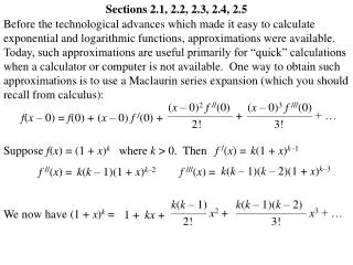
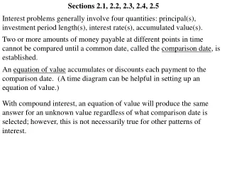
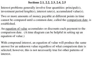
Sections 2.1, 2.2, 2.3, 2.4, 2.5 Interest problems generally involve four quantities: principal(s), investment period length(s), interest rate(s), accumulated value(s). Two or more amounts of money payable at different points in time cannot be compared until a common date, called the comparison date, is established. An equation of value accumulates or discounts each payment to the comparison date. (A time diagram can be helpful in setting up an equation of value.) With compound interest, an equation of value will produce the same answer for an unknown value regardless of what comparison date is selected; however, this is not necessarily true for other patterns of interest.
In return for a payment of $1200 at the end of 10 years, a lender agrees to pay $200 immediately, $400 at the end of 6 years, and a final amount at the end of 15 years. Find the amount of the final payment at the end of 15 years if the nominal rate of interest is 9% converted semiannually. Time Diagram: $200 $400 $X Lender Borrower 0 1 2 3 4 5 6 7 8 9 10 11 12 13 14 15 $1200 present (Time periods are counted in half-years, since interest is converted semiannually.) Equation of Value: v = 1 / (1 + 0.045) 200 + 400v12 + Xv30 = 1200v20
1200v20– 200 – 400v12 X = ————————— = v30 $231.11 In return for payments of $5000 at the end of 3 years and $4000 at the end of 9 years, an investor agrees to pay $1500 immediately and to make an additional payment at the end of 2 years. Find the amount of the additional payment if i(4) = 0.08. $1500 $X Time Diagram: Investor Borrower 0 1 2 3 4 5 6 7 8 9 10 $5000 $4000 Equation of Value: (Time periods are counted in quarter-years, since interest is converted quarterly.) v = 1 / (1 + 0.02) 1500 + Xv8 = 5000v12 + 4000v36 X = $5159.24
Consider the graphs of f(x) = x– 1 and f(x) = lnx . y = x– 1 y We find that for any x > 0, x – 1 lnx y = lnx x (1,0) Now, suppose a1 , a2 , … , an are all positive. Let T = a1 a2 … an , and let yi = ai / T1/n for each i = 1, 2, …, n. Then, y1 y2 … yn = , and ln(y1 y2 … yn) = . Also, we see that 1 0 (y1– 1) + (y2– 1) + … + (yn– 1) ln(y1) + ln(y2) + … + ln(yn) = ln(y1 y2 … yn) = 0.
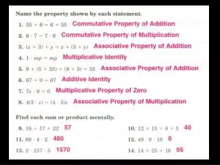
We now have that (y1– 1) + (y2– 1) + … + (yn– 1) 0 y1 + y2 + … + yn ——————— 1 n y1 + y2 + … + ynn a1 + a2 + … + an ——————— 1 T1/nn a1 + a2 + … + an ——————— (a1a2…an)1/n n In Section B of Appendix C (page 593), find the definition of the arithmetic mean and the geometric mean. Then observe that we have proven that that the arithmetic mean must always be greater than or equal to the geometric mean (assuming of course only positive values).
Amounts $500, $800, and $1000 are to be paid at respective times 3 years from today, 5 years from today, and 11 years from today. Suppose we would like to find the number of years t from today when one single payment of $500 + $800 + $1000 = $2300 would be equivalent to the individual payments made separately. If the rate of interest per annum is known to be i, then v = 1 / (1 + i), and the equation of value is 2300vt = 500v3 + 800v5 + 1000v11 In general, suppose amounts s1 , s2 , … , sn are to be paid at respective times t1 , t2 , … , tn . Also suppose we would like to find the time t when one single payment of s1 + s2 + … + sn would be equivalent to the individual payments made separately. If v = 1 / (1 + i) is known, then the equation of value is t1t2tn (s1 + s2 + … + sn)vt = s1v + s2v + … + snv (Observe what must be done to find an exact formula for the unknown value of t.)
t1t2tn (s1 + s2 + … + sn)vt = s1v + s2v + … + snv With the exact t, this is the true present value for the equivalent single payment. An approximate value of t can be obtained from the method of equated time. This method estimates t with s1t1 + s2t2 + … + sntn t = ————————— s1 + s2 + … + sn With the approximation t, the estimated present value for the equivalent single payment is t (s1 + s2 + … + sn)v In order to discover an interesting property about how the exact value of t and the estimate t compare, let us imagine that we have a list of numbers where s1 of the numbers are equal to v , s2 of the numbers are equal to v , etc. t1 t2
In order to discover an interesting property about how the exact value of t and the estimate t compare, let us imagine that we have a list of numbers where s1 of the numbers are equal to v , s2 of the numbers are equal to v , etc. t1 t2 s1t1 + s2t2 + … + sntn ————————— s1 + s2 + … + sn t Then v can be written as v = 1 —————— s1 + s2 + … + sn From Section B of Appendix C, we see that this is the geometric mean of the list of numbers. s1t1 s2t2 sntn v v … v This is the product of the list of numbers. t1t2tn s1v + s2v + … + snv —————————— s1 + s2 + … + sn t and v can be written as From Section B of Appendix C, we see that this is the arithmetic mean of the list of numbers. This is the average of the list of numbers.
Since the arithmetic mean of positive numbers must always be larger than the geometric mean, we have that t t v > v t1t2tn s1v + s2v + … + snv —————————— s1 + s2 + … + sn t > v t t1t2tn s1v + s2v + … + snv > (s1 + s2 + … + sn)v We now see that the true present value (on the left) will always be larger than the estimated present value (on the right). Consequently, the estimated time t from the method of equated time must be an overestimation.
Amounts $500, $800, and $1000 are to be paid at respective times 3 years from today, 5 years from today, and 11 years from today. The effective rate of interest is 4.5% per annum. (a) (b) Use the method of equated time to find the number of years t from today when one single payment of $500 + $800 + $1000 = $2300 would be equivalent to the individual payments made separately. s1t1 + s2t2 + … + sntn t = ————————— = s1 + s2 + … + sn (500)(3) + (800)(5) + (1000)(11) ————————————— = 2300 7.174 years Find the exact number of years t from today when one single payment of $500 + $800 + $1000 = $2300 would be equivalent to the individual payments made separately. With v = 1 / (1 + 0.045), the equation of value is 2300vt = 500v3 + 800v5 + 1000v11 500v3 + 800v5 + 1000v11 vt = —————————— = 2300 0.73752 t = 6.917 years
Given a particular rate of interest, how long will it take an investment to double? By solving (1 + i)n = 2, we find the exact solution n = ln(2) ——— ln(1 + i) 0.6931 ——— = ln(1 + i) 0.6931 i ——— ——— , i ln(1 + i) Observe that n 0.72 —— = i 72 —— . 100i and when i = 0.08 in the second factor, we have n This is called the rule of 72, and it gives amazingly accurate results for a wide range of interest rates! (See Table 2.1 on page 57 of the text.)
Suppose $2000 is invested at a rate of 7% compounded semiannually. (a) (b) (c) Find the length of time for the investment to double by using the exact formula. t = years 2000(1.035)2t = 4000 t = 10.074 years Find the length of time for the investment to double by using the rule of 72. 72/3.5 = 20.571 half years t = 10.286 years Find the length of time for the investment to be worth $3000 by using the exact formula. t = years 2000(1.035)2t = 3000 t = 5.893 years
Suppose it is the rate of interest i that is unknown in an equation of value. There are several methods available for solving for i, and depending on the type of situation, one method may be better suited than another. At what interest rate convertible semiannually would $500 accumulate to $800 in 4 years? When a single payment is involved, the method that works best is to solve for i directly in the equation of value (using exponential and logarithmic functions). 500(1 + j)8 = 800 1 + j = (8/5)1/8 j = (8/5)1/8 – 1 = 0.0605 i(2) = 2j = (2)(0.0605) = 0.0121 = 12.1%
At what effective interest rate would the present value of $1000 at the end of 3 years plus $2000 at the end of 6 years be equal to $2700? When multiple payments are involved, the equation of value is generally a polynomial, and the method to solve for i is one for obtaining the roots of a polynomial. Sometimes this can be done using the quadratic formula. 1000v3 + 2000v6 = 2700 2000v6 + 1000v3– 2700 = 0 20v6 + 10v3– 27 = 0 We are only interested in v > 0, and the only positive root from the quadratic formula is v3 = , from which we obtain v = 0.9385 0.9791. v = 1 / (1 + i) = 0.9791 i = 0.02145
At what interest rate convertible semiannually would an investment of $1000 immediately and $2000 three years from now accumulate to $5000 ten years from now? If we let j = i(2)/2, then the equation of value is 1000(1 + j)20 + 2000(1 + j)14– 5000 = 0 When solving the equation of value involves a polynomial whose roots cannot be obtained easily, an iterative procedure can be used. The use of a computer generally makes an iterative procedure much easier to use. Use the Excel file Interest_Solver to find the solution to this equation of value as follows:
Type the formula =1000*(1+j)^20+2000*(1+j)^14-5000 in cell A5. Select options Tools > Solver to solve the equation of value as indicated below (and if necessary, first use options Tools > Add-Ins) You should find that j = 0.032178 is the solution, from which we have i = 0.065391. Section 2.7 of the textbook discusses some of the ambiguous interpretations of words used in the “real world” versus the precise meanings used in mathematics.