STA 291 Lecture 20
330 likes | 349 Vues
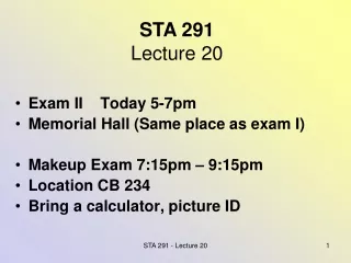
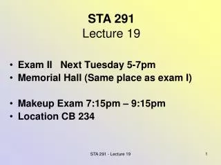
STA 291 Lecture 20. Exam II Today 5-7pm Memorial Hall (Same place as exam I) Makeup Exam 7:15pm – 9:15pm Location CB 234 Bring a calculator, picture ID. Exam II Covers …. Chapter 9 10.1; 10.2; 10.3; 10.4; 10.6 12.1; 12.2; 12.3; 12.4

STA 291 Lecture 20
E N D
Presentation Transcript
STA 291Lecture 20 • Exam II Today 5-7pm • Memorial Hall (Same place as exam I) • Makeup Exam 7:15pm – 9:15pm • Location CB 234 • Bring a calculator, picture ID STA 291 - Lecture 20
Exam II Covers … • Chapter 9 • 10.1; 10.2; 10.3; 10.4; 10.6 • 12.1; 12.2; 12.3; 12.4 • Formula sheet; normal table; t-table will be provided. STA 291 - Lecture 20
Example: • Smokers try to quit smoking with Nicotine Patch or Zyban. • Find the 95% confidence intervals STA 291 - Lecture 20
Example • To test a new, high-tech swimming gear, a swimmer is asked to swim twice a day, one with the new gear, one with the old. • The difference in time is recorded: Time(new) – time(old) = -0.08, -0.1, 0.02, …. -0.004. There were a total of 21 such differences. Q: is there a difference? STA 291 - Lecture 20
First: we recognize this is a problem with mean mu. • And we compute the average X bar= -0.07 • SD = 0.02 • 90% confidence interval is: STA 291 - Lecture 20
Plug-in the values into formula STA 291 - Lecture 20
What is the ?? Value. • It would be 1.645 if we knew sigma, the population SD. But we do not, we only know the sample SD. So we need T-adjustment. • Df= 21 -1 = 20 • ??=1.725 STA 291 - Lecture 20
Confidence interval for mu • For continuous type data, often the parameter is the population mean, mu. • Chap. 12.1 – 12.4 STA 291 - Lecture 20
Chap. 12.1 – 12.4:Confidence Interval for mu • The random interval between Will capture the population mean, mu, with 95% probability • This is a confidence statement, and the interval is called a 95% confidence interval • We need to know sigma. STA 291 - Lecture 20
confidence level 0.90, =1.645 • confidence level 0.95 =1.96 • confidence level 0.99 =2.575 • Where do these numbers come from? (same number as the confidence interval for p). • They are from normal table/web STA 291 - Lecture 20
“Student” t - adjustment • If sigma is unknown, (often the case) we may replace it by s (the sample SD) but the value Z (for example z=1.96) needs adjustment to take into account of extra variability introduced by s • There is another table to look up: t-table or another applet • http://www.socr.ucla.edu/Applets.dir/Normal_T_Chi2_F_Tables.htm STA 291 - Lecture 20
Degrees of freedom, n-1 • Student t - table is keyed by the df – degrees of freedom • Entries with infinite degrees of freedom is same as Normal table • When degrees of freedom is over 200, the difference to normal is very small STA 291 - Lecture 20
With the t-adjustment, we do not require a large sample size n. • Sample size n can be 25, 18 or 100 etc. STA 291 - Lecture 20
Example: Confidence Interval • Example: Find and interpret the 95% confidence interval for the population mean, if the sample mean is 70 and the pop. standard deviation is 12, based on a sample of size n = 100 First we compute =12/10= 1.2 , 1.96x 1.2=2.352 [ 70 – 2.352, 70 + 2.352 ] = [ 67.648, 72.352] STA 291 - Lecture 20
Example: Confidence Interval • Now suppose the pop. standard deviation is unknown (often the case). Based on a sample of size n = 100 , Suppose we also compute the s = 12.6 (in addition to sample mean = 70) First we compute =12.6/10= 1.26 , From t-table 1.984 x 1.26 = 2.4998 [ 70 – 2.4998, 70 + 2.4998 ] = [ 67.5002, 72.4998] STA 291 - Lecture 20
Confidence Interval: Interpretation • “Probability” means that “in the long run, 95% of these intervals would contain the parameter” i.e. If we repeatedly took random samples using the same method, then, in the long run, in 95% of the cases, the confidence interval will cover the true unknown parameter • For one given sample, we do not know whether the confidence interval covers the true parameter or not. (unless you know the parameter) • The 95% probability only refers to the method that we use, but not to the individual sample STA 291 - Lecture 20
Confidence Interval: Interpretation • To avoid the misleading word “probability”, we say: “We are 95% confident that the interval will contain the true population mean” • Wrong statement: “With 95% probability, the population mean is in the interval from 3.5 to 5.2” Wrong statement: “95% of all the future observations will fall within 3.5 to 5.2”. STA 291 - Lecture 20
Confidence Interval • If we change the confidence level from 0.95 to 0.99, the confidence interval changes Increasing the probability that the interval contains the true parameter requires increasing the length of the interval • In order to achieve 100% probability to cover the true parameter, we would have to increase the length of the interval to infinite -- that would not be informative, not useful. • There is a tradeoff between length of confidence interval and coverage probability. Ideally, we want short length and high coverage probability (high confidence level). STA 291 - Lecture 20
Different Confidence Coefficients • In general, a confidence interval for the mean, has the form • Where z is chosen such that the probability under a normal curve within z standard deviations equals the confidence level STA 291 - Lecture 20
Different Confidence Coefficients • We can use normal Table to construct confidence intervals for other confidence levels • For example, there is 99% probability of a normal distribution within 2.575 standard deviations of the mean • A 99% confidence interval for is STA 291 - Lecture 20
Error Probability • The error probability (α) is the probability that a confidence interval does not contain the population parameter -- (missing the target) • For a 95% confidence interval, the error probability α=0.05 • α = 1 - confidence level or confidence level = 1 – α STA 291 - Lecture 20
Different Confidence Levels STA 291 - Lecture 20
If a 95% confidence interval for the population mean, turns out to be [ 67.4, 73.6] What will be the confidence level of the interval [ 67.8, 73.2]? STA 291 - Lecture 20
Choice of sample size • In order to achieve a margin of error smaller than B, (with confidence level 95%), how large the sample size n must we get? STA 291 - Lecture 20
Choice of Sample Size • So far, we have calculated confidence intervals starting with z, n and • These three numbers determine the error bound B of the confidence interval • Now we reverse the equation: • We specify a desired error bound B • Given z and , we can find the minimal sample size n needed for achieve this. STA 291 - Lecture 20
Choice of Sample Size • From last page, we have • Mathematically, we need to solve the above equation for n • The result is STA 291 - Lecture 20
Example • About how large a sample would have been adequate if we merely needed to estimate the mean to within 0.5, with 95% confidence? • (assume • B=0.5, z=1.96 • Plug into the formula: STA 291 - Lecture 20
Choice of sample size • The most lazy way to do it is to guess a sample size n and • Compute B, if B not small enough, then increase n; • If B too small, then decrease n STA 291 - Lecture 20
For the confidence interval for p • Often, we need to put in a rough guess of p (called pilot value). Or, conservatively put p=0.5 STA 291 - Lecture 20
Suppose we want a 95%confidence error bound B=3% (margin of error + - 3%). Suppose we do not have a pilot p value, so use p = 0.5 So, n = 0.5(1-0.5) [ 1.96/0.03]^2=1067.11 STA 291 - Lecture 20
Attendance Survey Question • On a 4”x6” index card • Please write down your name and section number • Today’s Question: Which t-table you like better? STA 291 - Lecture 20
Facts About Confidence Intervals I • The width of a confidence interval • Increases as the confidence level increases • Increases as the error probability decreases • Increases as the standard error increases • Decreases as the sample size n increases STA 291 - Lecture 20
