Download

1 / 82
980 likes | 1.39k Vues
Chapter 3 Graphs, Trees, and Tours. Presented by Qibin Cai. Overview. Terminology in graph theory. Trees - Minimum spanning tree (MST) - Shortest path tree (SPT). Tours - TSP tours. Building trees Kruskal’s algorithm Prim’s algorithm Dijkstra’s algorithm

E N D
Chapter 3Graphs, Trees, and Tours Presented by Qibin Cai
Overview • Terminology in graph theory • Trees • - Minimum spanning tree (MST) • - Shortest path tree (SPT) • Tours • - TSP tours
Building trees Kruskal’s algorithm Prim’s algorithm Dijkstra’s algorithm Prim-Dijkstra algorithm Building tours Nearest-neighbor algorithm Improved nearest-neighbor heuristic - Divide and conquer strategy Overview cont’d
Terminology • What is a graph? • Observation: A graph is a set of points in a plane (or in 3-space) and a set of line segments (possibly curved), each of which either joins two points or joins a point to itself.
Some definitions • Graphs • A,B,C etc. are vertices(nodes) • (A,X), (X,Y) etc. are edges • P,Q,Z is a cycle • Degree of a node is the number of edges at the node • Degree Y =3, degree C=1 C B P Y Q X A Z D
Terminology cont’d • Definition in mathematical language? • A graph G = (V, E) is a mathematical structure consisting of two sets V and E. The elements of V are called vertices (or nodes), and the elements of E are called edges. • Digragh : a directed graph
Terminology cont’d • Endpoints : a set of one or two vertices associated to each edge. • Loop: an edge where both endpoints are the same. Also called a self-loop. • Parallel edges: a collection of two or more edges having identical end. Also called a multi-edge.
Terminology cont’d • A graph is simple if it has no loops or parallel edges. • Most of our discussions will involve simple graphs. Sometimes, when we considering reliability, we will introduce parallel edges if the network has parallel links.
Terminology cont’d • The degree of a node: the number of edges in the graph that have the node as an endpoint (plus twice the number of self-loops). • Indegree • Outdegree
Terminology cont’d • Adjacent vertices: Two nodes are adjacent if there is an edge that has them as endpoints. • Incidence: The relationship between an edge and its endpoints.
Terminology cont’d • Walk from vertex u to vertex v: an alternating sequence of vertices and edges, representing a continuous traversal from vertex u to vertex v. • Trail: a walk with no repeated edges. • Path: a walk with no repeated vertices.
Terminology cont’d • Cycle: a closed path with at least an edge. • Connected graph: a graph in which every pair of distinct vertices has a walk between them.
Terminology cont’d • Subgraph: A graph G’=(N’,A’) is a subgraph of G=(N,A) if N’ N and A’ A. • Component: a maximal connected subgraph of a graph.
Terminology cont’d • Isomorphism: Two graphs G1 and G2 are isomorphic if there is a 1-to-1 mapping f: v1 -> v2 such that (v1, v2) E1 if and only if (f(v1), f(v2)) E2.
Trees • Tree: a connected, simple graph without cycles. • Star: a tree in which only 1 node has degree greater than 1. • Chain: a tree in which no node has degree greater than 2. • Any tree with n nodes has n-1 edges.
Trees • A tree is a connected simple graph with no cycles e.g. C B P Q Y X A Z D
Star • A tree is a star if only 1 node has degree >1 C B P Y Q X Z A D
Chains • A chain is a tree with no nodes of degree >2 C B P Q Y X A Z D
Weighted Graph • A graph G is weighted if there is a value associated with each edge (e.g. link speed, cost, etc.) • Weight of the edge ei = w(ei) • We often denote this graph (G, w). If G’ is any subgraph of G, then w(G’) = • To optimise a connected graph find the graph with the minimum weight • The Minimal Spanning Tree (MST)
Minimal Spanning Trees • Let G be a connected weighted graph. • A spanning subgraph includes all the nodes of G. • A tree T is a spanning tree of G if T is a spanning subgraph of G. • MST: A spanning tree of G whose total edge-weight is a minimum.
Finding the MST • Two algorithms Kruskal and Prim • Kruskal achieves the MST by starting with a graph and cutting out edges • Prim • starts by selecting a node, • adding the “least expensive edge” • iterates until tree is built
Use of MSTs • Small design problems - few nodes • Highly reliable links with low “downtime” • or network can tolerate unreliability • Nodes ‘v’ reliability • As the number of nodes increases reliability decreases (exponentially!)
Kruskal’s Algorithm (1956) • 1. Check that the graph G is connected. If it is not connected, abort. • 2. Sort the edges of the graph G in ascending order of weight. • 3. Mark each node as a separate component. • 4. Examine each of the sorted edges: if the edge connects two separate components, add it ; otherwise, discard.
Prim’s Algorithm (1957) • Input : a weighted connected graph G=(N,E). • Output : a minimum spanning tree T. • U = set of all nodes in MST • V = set of all nodes that are NOT yet in MST, but they’re adjacent to nodes in U.
Prim’s Algorithm (cont’d) • 1. Place any node in U, and update V . • 2. Find the edge with smallest weight that connects a node in V to a node in U • 3. Add that edge to the tree, and update U & V. • 4. Repeat 2 & 3 until all nodes are included, i.e., | U | = | N |.
How to use Delite to Calculate MST’s • Invoke the code for Prim’s algorithm from the Design menu. • Select to produce a trace file • Demonstration
Tree Designs • Overview • Squareworld • Coordinate systems: • - V & H • - L & L • MSTs do not scale • Definitions: hops(n1,n2),
Square World • We will create a little world with several properties that make it a nice place to work on network design problem. • The world is 1000 miles by 1000 miles. • 1 type of transmission line with a capacity of 1,000,000 bps. • Given 2 sites, S1 at location (X1, Y1) and S2 at location (X2,Y2), the cost of a link between them is ($1000 + $10 x d) / month where
2 Coordinate Systems We will use a problem generator to set up a series of network design problems. Before we can do this, we need to know something about the methods of locating sites are used in the real world. • Vertical and horizontal (V&H) - a grid of lines, or more accurately curves is drawn. - allows for a simplified computation of distances. • Latitude and longitude (L&L) - defined for all locations on the surface of the earth. - The distance calculation is essentially an exercise in spherical geometry.
MSTs Do Not scale • Why? First look at an example. • Figure 3.2 (An MST for 5 nodes in square world) N2 N1 N5 N4 N3 MAX_UTIL=0.6%
Figure 3.3 (An MST for 10 nodes in square world) N6 N2 N7 N10 N9 N1 N5 N4 N8 N3 MAX_UTIL=2.5% The network is beginning to have a leggy look, which means that the traffic is taking a circuitous route between its source and destination. To qualify the legginess in the network, we make the following definition.
Definitions 3.17 - The number of hops between node n1 and n2 is the number of edges in the path chosen by the routing algorithm for the traffic flowing from n1 to n2. Denoted by hops (n1,n2) Definitions 3.18 - The average number of hops in a network is: Denoted by Two Definitions
MSTs Do Not scale (cont’d) • We summarize the values of as below: Number of nodes 5 1.8 10 3.1778 20 4.4158 50 8.5159 100 13.9479 #hops grow past a reasonable level, and MSTs are not good solutions as # nodes and the traffic grow. Then we will consider if we can design better trees.
Shortest-Path Trees (SPT) • Definition 3.19 Given a weighted graph (G,W) and nodes n1 and n2, the shortest path from n1 to n2 is a path P such that is a minimum. • Definition 3.20 Given a weighted graph (G,W) and a node n1, a shortest – path tree rooted at n1 is a tree T such that, for any other node n2 G, the path from n1 to n2 in the tree T is a shortest path between the nodes.
Dijkstra’s Algorithm • 1. Mark every node as unscanned and give each node a label of • 2. Set the label of the root to 0 and the predecessor of the root to itself. The root will be the only node that is its own predecessor.
Dijkstra’s Algorithm (cont’d) • 3. Loop until you have scanned all the nodes. -Find the node n with the smallest label. Since the label represents the distance to the root we call it d_min. -Mark the node as scanned. -Scan all the adjacent nodes m and see if the distance to the root through n is better than the distance stored in the label of m. If it is, update the label and update pred[m]=n. • 4. When the loop finishes, we have a tree stored in pred format rooted at root.
SPT vs. MST • Lower utilization of the links • More cost • Important: Smaller average number of hops Actually we will compare star (a kind of SPT) with MST, because …
Star vs. MST SPT vs. MST • If we run Dijkstra’s algorithm on a sparse graph, we will get a tree with a fair number of nodes not connected directly to the root. • If we run Dijkstra’s algorithm on a complete graph (exactly what we’re studying now), then we usually get a star.
Star vs. MST (cont’d) Design name MAX_UTIL Cost MST 13.9479 0.493 $325.516 Star 1.9800 0.09 $453.861 Prim’s algorithm produces much shorter paths but can produce very expensive networks. SPT is not good, either. Is there some middle ground between MST and SPT?
Prim – Dijkstra Trees Algorithm : Label 1) Prim’s: 2) Dijkstra’s: 3) Prim-Dijkstra’s:
Prim – Dijkstra Trees (cont’d) • If , we build a MST. • If , we build a SPT. • The delay, and cost for various Prim-Dijkstra trees. Design Link delay Cost 0(MST) N0 13.9479 0.3066 $325,516 0.1 N1 10.5717 0.1451 $280,162 0.2 N2 7.8640 0.1067 $247,217 0.3 N3 6.7762 0.0913 $243,551 0.4 N4 5.6679 0.0746 $248,650 0.5 N5 4.6303 0.0598 $253,579 0.6 N6 3.7063 0.0467 $273,742 0.7 N7 3.0186 0.0380 $295,012 0.8 N8 2.2879 0.0277 $378,792 0.9 N9 1.9800 0.0233 $453,861 If we have such a large set of designs shown in the table, how to select the best?
Dominance among Designs • If we have a large set of designs, the problem is to decide which merit consideration and which should be discarded. • To help us do this we impose a partial ordering on the designs.
Dominance among Designs(cont’d) • Definition 3.21: Given a set S and an operator that maps S x S {TRUE,FALSE}, then we call S a partially ordered set, or poset, if 1) For any s S, s s is FALSE. 2) For any s1, s2 S, s1 s2, if s1 s2 is TRUE, then s2 s1 is FALSE. 3) If s1 s2 and s2 s3 are TRUE, then s1 s3 is TRUE.
Dominance among Designs(cont’d) • Definition 3.22: Suppose design D1 has cost C1 and performance P1. Suppose design D2 has cost C2 and performance P2. We will say D1 dominates D2, or D1 D2, if C1 < C2 and P1 > P2.
Dominance among Designs(cont’d) Design Dominates Link delay Cost N0 0.3066 $325,516 N1 N0 0.1451 $280,162 N2 N0,N1 0.1067 $247,217 N3 N0,N1,N2 0.0913 $243,551 N4 N0,N1 0.0746 $248,650 N5 N0,N1 0.0598 $253,579 N6 N0,N1 0.0467 $273,742 N7 N0 0.0380 $295,012 N8 0.0277 $378,792 N9 0.0233 $453,861
Dominance among Designs(cont’d) • Show dominance relationships as a directed graph: A directed graph is a graph G=(V,E) in which each edge e has been given an orientation. If the edge has endpoints v1 and v2, we shall denote the edge e=(v1,v2) if the orientation of v1 is the source vertex.
Dominance among Designs(cont’d) • Think of the designs (N0,N1,N2,…,N9) as the nodes of a graph. • A directed edge runs from Ni to Nj if Ni Nj. • We can see we don’t want to consider N0, N1, or N2. N9 N8 N3 N2 N5 N1 N4 N7 N6 N0
Further Analysis ofPrim-Dijkstra Trees • Given a pair of nondominating designs S1 and S2, 1 must be cheaper and 1 must have lower delay. • After rejecting the dominated designs, we still have 7 designs left to choose from. One way to clarify their differences further is to discuss the marginal cost of delay: C1 - C2 P2 - P1
Using Delite to ProducePrim-Dijkstra Trees • Unlike Prim’s algorithm, the choice of the node at the center of the tree is important in the Prim-Dijkstra algorithm. • The value of . • Create trace file.