Download
1 / 40
440 likes | 529 Vues
Introduction to Bayesian Statistics. Jeff Witmer. 24 February 2016. A semester ’ s worth of material in just a few dozen slides. Why Bayes?. Because Bayes answers the questions we really care about. Pr(I have disease | test +) vs Pr(test + | disease).

E N D
Introduction to Bayesian Statistics Jeff Witmer 24 February 2016 A semester’s worth of material in just a few dozen slides.
Why Bayes? Because Bayes answers the questions we really care about. Pr(I have disease | test +) vs Pr(test + | disease) Pr(A better than B | data) vs Pr(extreme data | A=B) Bayes is natural (vs interpreting a CI or a P-value) Note: blue = Bayesian, red = frequentist
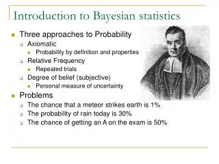
You are waiting on a subway platform for a train that is known to run on a regular schedule, only you don't know how much time is scheduled to pass between train arrivals, nor how long it's been since the last train departed. As more time passes, do you (a) grow more confident that the train will arrive soon, since its eventual arrival can only be getting closer, not further away, or (b) grow less confident that the train will arrive soon, since the longer you wait, the more likely it seems that either the scheduled arrival times are far apart or else that you happened to arrive just after the last train left – or both.
If you choose (a), you're thinking like a frequentist. If you choose (b), you're thinking like a Bayesian. from Floyd Bullard
An opaque jar contains thousands of beads (but obviously a finite number!). You know that all the beads are either red or white but you have no idea at all what fraction of them are red. You begin to draw beads out of the bin at random without replacement. You notice that all of the first several beads have been red. As you observe more and more red beads, is the conditional probability (i.e., conditional upon the previous draws' colors) of the next bead being red (a) decreasing, as it must, since you're removing red beads from a finite population, or (b) increasing, because you initially didn’t know that there would be so many reds, but now it seems that the jar must be mostly reds.
If you choose (a), you're thinking like a frequentist. If you choose (b), you're thinking like a Bayesian. from Floyd Bullard
Probability Limiting relative frequency: A nice definition mathematically, but not so great in practice. (So we often appeal to symmetry…) What if you can’t get all the way to infinity today? What if there is only 1 trial? E.g., P(snow tomorrow) What if appealing to symmetry fails? E.g., I take a penny out of my pocket and spin it. What is P(H)?
Subjective probability Prob = Odds = Fair die Event Prob Odds even # 1/2 1 [or 1:1] X > 2 2/3 2 [or 2:1] roll a 2 1/6 1/5 [or 1/5:1 or 1:5] Persi Diaconis: "Probability isn't a fact about the world; probability is a fact about an observer's knowledge."
Bayes’ Theorem P(a|b) = P(a,b)/P(b) P(b|a) = P(a,b)/P(a) P(a,b) = P(a)P(b|a) Thus, P(a|b) = P(a,b)/P(b) = P(a)P(b|a)/P(b) But what is P(b)? P(b) = Σ P(a,b) = Σ P(a)P(b|a) a a Thus, P(a|b) = Where a* means “any value of a”
P(a|b) = P(a|b) P(a) P(b|a) posterior (prior) (likelihood) Bayes’ Theorem is used to take a prior probability, update it with data (the likelihood), and get a posterior probability.
Medical test example. Suppose a test is 95% accurate when a disease is present and 97% accurate when the disease is absent. Suppose that 1% of the population has the disease. What is P(have the disease | test +)?
Typical statistics problem: There is a parameter, θ, that we want to estimate, and we have some data. Traditional (frequentist) methods: Study and describe P(data | θ). If the data are unlikely for a given θ, then state “that value of θ is not supported by the data.” (A hyp. test asks whether a particular value of θ might be correct; a CI presents a range of plausible values.) Bayesian methods: Describe the distribution P(θ | data). A frequentist thinks of θ as fixed (but unknown) while a Bayesian thinks of θ as a random variable that has a distribution. Bayesian reasoning is natural and easy to think about. It is becoming much more commonly used.
If Bayes is so great, why hasn’t it always been popular? (1) Without Markov Chain Monte Carlo, it wasn’t practical. (2) Some people distrust prior distributions, thinking that science should be objective (as if that were possible). Bayes is becoming much more common, due to MCMC. E.g., Three recent years worth of J. Amer. Stat. Assoc.“applications and case studies” papers: 46 of 84 papers used Bayesian methods (+ 4 others merely included an application of Bayes’ Theorem).
What is MCMC? We want to find P(θ | data), which is equal to P(θ)*P(data |θ)/P(data) and is proportional to P(θ)*P(data | θ), which is "prior*likelihood”. But to use Bayesian methods we need to be able to evaluate the denominator, which is the integral of the numerator, integrated over the parameter space. In general, this integral is very hard to evaluate. Note: There are two special cases in which the mathematics works out: for a beta-prior with binomial-likelihood (which gives a beta posterior) and for a normal prior with normal likelihood (which gives a normal posterior).
But for general cases the mathematics is not tractable. However, MCMC has given us a way around this. We don't need to evaluate any integral, we just sample from the distribution many times (e.g., 50K times) and find (estimate) the posterior mean, middle 95%, etc., from that. How does MCMC work? It is based on the Metropolis algorithm… Note: These days we typically use Gibbs sampling, which is a variation on Metropolis. Old software: BUGS – Bayes Using Gibbs Sampling Newer software: JAGS – Just Another Gibbs Sampler Newest software: Stan – uses Hamiltonian Monte Carlo
Skip this slide… Beta random variables where where Run BetaPlot.R….
Binomial (Bernoulli) data and a Beta prior Posterior Prior * Likelihood if there are z successes in n trials Thus post This is a Beta(a+z, b+n-z)
See Effect on posterior of large n.R. Data: 1 success in 4 trials.
See BernBetaExampleLoveBlindMen.R. Data: 16 of 36 men correctly identify their partner.
See Run Jags-Ydich-Xnom1subj-MbernBeta-LoveBlindMen.R which uses MCMC – and gives similar results P(0.29 < θ < 0.60) = 0.95
Does the prior make sense? Does it give rise to reasonable data? Let θ = % OC veggies. Prior: I think that θ might be around 0.20 and my prior is worth 20 observations. This corresponds to a prior on θ that is Beta(4.6, 15.4). Does that prior give rise to reasonable data? Simulate 2000 times getting samples of n=25:
Comparing 2 proportions. Love is Blind data. 98% prob women better Men: 16/36 Women: 25/36 Frequentist P-value = 0.03.
Overall, guards shoot FTs better than centers. However, in 2014-15 center Willie Cauley-Stein made 61.7% (79/128) while guard Quentin Snider made 55.3% (21/38). Is Snider really worse? A Bayesian analysis says “P(Snider is better) = 87.5%.” So far in 2015-16 Cauley-Stein has made 58.6% (41/70) while Snider has made 71.7% (33/46). Obs diff = 0.553 – 0.617
Skip this slide… basketball data comparing men and women See rpubs.com/jawitmer/68406 and rpubs.com/jawitmer/99006
MCMC can handle many parameters. 928 parameters See rpubs.com/jawitmer/64891
Normal data – comparing 2 means Myocardial blood flow (ml/min/g) for two groups. Normoxia: 3.45, 3.09, 3.09, 2.65, 2.49, 2.33, 2.28, 2.24, 2.17, 1.34 Hypoxia: 6.37, 5.69, 5.58, 5.27, 5.11, 4.88, 4.68, 3.50 P(1.76 < µ2 - µ1 < 3.51) = 0.95. [The standard/frequentist 95% CI is (1.85, 3.39) ] See rpubs.com/jawitmer/154977
Normal data – comparing 2 means See the BEST website: http://www.sumsar.net/best_online/ There is also an easy-to-use R package: Bayesian First Aid with(ExerciseHypoxia, t.test(MBF ~ Oxygen)) is changed to with(ExerciseHypoxia, bayes.t.test(MBF ~ Oxygen))
Lognormal vs Normal With MCMC, we don’t need to assume a normality for data. Use y[i] ~dlnorm() instead of y[i] ~ dnorm().
Regression – How to handle outliers… Outlier 95% CI for slope: (1.12, 1.69) or (1.14, 1.60)
We can use a t as the likelihood function (vs the usual normal distribution) 95% HDI for slope: (1.13, 1.67)
Kruschke, John K. (2015). Doing Bayesian Data Analysis: A Tutorial with R, JAGS, and Stan. 2nd Ed. Academic Press. McGrayne, Sharon Bertsch (2011). The Theory that Wouldn’t Die. Yale University Press.