
So far…
So far… . Signals to sequences Convolution between sequences and is defined as or Correlation between two sequences and Impulse response of a system Where is the unit sample or impulse response of the LTI system System is stable if

So far…
E N D
Presentation Transcript
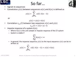
So far… • Signals to sequences • Convolution between sequences and is defined as or • Correlation between two sequences and • Impulse response of a system • Where is the unit sample or impulse response of the LTI system • System is stable if • In general, the response sequence to the input sequence can be re-written as Matone: An Overview of Control Theory and Digital Signal Processing (4)
So far… • Differential to difference equations • General form of a difference equation • MATLAB’s filter command to numerically solve difference equations: >> y = filter(b, a, x) • In particular the impulse response of a system can be found >> h = filter(b, a, delta) Matone: An Overview of Control Theory and Digital Signal Processing (4)
Digital Signal Processing 2 • In the analog domain, the Laplace transform L • Relates time-functions to frequency-dependent functions • For the digital domain, the Z transform • Relates time-sequences to (a different, but related type of) frequency-dependent function Matone: An Overview of Control Theory and Digital Signal Processing (4)
The Z Transform • This discrete-time equivalent of the Laplacetransform is defined as where is the complex frequency. • The values of for which the sum converges define a region in the -plane referred to as the region of convergence (ROC). Matone: An Overview of Control Theory and Digital Signal Processing (4)
Region of convergence (ROC) ROC The set of z values for which exists is called the region of convergence (ROC) Matone: An Overview of Control Theory and Digital Signal Processing (4)
The Z Transform This transformation is useful in Solving constant coefficient difference equations Evaluating the response of an LTI system to a given input, and Designing linear filters Matone: An Overview of Control Theory and Digital Signal Processing (4)
Geometric series: Example ROC Transfer function: zero at the origin, pole at 1 Let . Find its Z transform and its ROC. or Matone: An Overview of Control Theory and Digital Signal Processing (4)
Example ROC Transfer function: zero at the origin, pole at 2 Let Find its Z transform and its ROC. or Matone: An Overview of Control Theory and Digital Signal Processing (4)
Example Pole at Zero at origin o Let . Find its Z transform and its ROC. Matone: An Overview of Control Theory and Digital Signal Processing (4)
In general Many of the signals in DSP have Z transforms that are rational (ratio of two polynomials) functions of : where is the k-th pole and is the l-th zero of . Each pole is indicated by an ”x” and each zero by an “o” in the -plane. Matone: An Overview of Control Theory and Digital Signal Processing (4)
Special properties of the Z Transform • Convolution • Given two sequences and , their time-domain convolution becomes a multiplication process in the frequency domain • Sample shifting Matone: An Overview of Control Theory and Digital Signal Processing (4)
(Some) Z Transform pairs Matone: An Overview of Control Theory and Digital Signal Processing (4)
And back to sequences: The Inverse ZTransform If Just like in the Laplace domain Use the partial fraction method to reduce a complex to simpler parts. Use the table of transform pairs to determine the sequence. In general Matone: An Overview of Control Theory and Digital Signal Processing (4)
Example Using the table of transform pairs Compute the inverse Z-transform of Sol: Re-write in terms of powers of . At the MATLAB prompt >> b=[0 1];a=[3 -4 1]; >> [R,p,C]=residuez(b,a) R = 0.5000 -0.5000 p = 1.0000 0.3333 C = [] Matone: An Overview of Control Theory and Digital Signal Processing (4)
Example Compute the inverse Z-transform of Sol: Using MATLAB to do the partial fraction >> b = 1; a = poly([0.9, 0.9, -0.9]) a = 1.0000 -0.9000 -0.8100 0.7290 Matone: An Overview of Control Theory and Digital Signal Processing (4)
Example >> [R,p,C]=residuez(b,a) R = 0.2500 0.2500 + 0.0000i 0.5000 - 0.0000i p = -0.9000 0.9000 + 0.0000i 0.9000 - 0.0000i C = [] Matone: An Overview of Control Theory and Digital Signal Processing (4)
Example Sample shifting Using the Z Transform pair table Matone: An Overview of Control Theory and Digital Signal Processing (4)
Exercise Determine the Z-transform of the impulse response Matone: An Overview of Control Theory and Digital Signal Processing (4)
Exercise Determine the Z-transform of the impulse response Sol: Using the sample shift property Matone: An Overview of Control Theory and Digital Signal Processing (4)
System function The system function is simply the Ztransform of the impulse response of the system This means that, given input the output is Matone: An Overview of Control Theory and Digital Signal Processing (4)
System function from a difference equation When an LTI system is represented by the difference equation it can be shown that where Matone: An Overview of Control Theory and Digital Signal Processing (4)
System function and MATLAB implementation The MATLAB implementation, given The impulse response is simply >> h = filter(b, a, delta) While the response to input is >> y = filter(b, a, x) Matone: An Overview of Control Theory and Digital Signal Processing (4)
For example Given the LTI system represented by the difference equation, the determine the impulse response . Sol: let’s find the system function first. Taking the Z transform Matone: An Overview of Control Theory and Digital Signal Processing (4)
Taking the inverse transform Let’s verify with MATLAB >> b = [1]; a = [1 -0.9]; >> h = filter(b,a,delta); and lets plot the two responses. Matone: An Overview of Control Theory and Digital Signal Processing (4)
ex411.m Matone: An Overview of Control Theory and Digital Signal Processing (4)
To recap The Z transform is the digital equivalent of the Laplace transform: • It facilitates the solving of constant coefficient difference equations • It allows to easily evaluate the system’s response • It is critical in designing linear filters MATLAB commands used • filter, residuez Matone: An Overview of Control Theory and Digital Signal Processing (4)
A different transform: DTFT • A very different but very useful representation of a sequence or system is the Discrete-time Fourier Transform (DTFT) • Setting in the -transform where is the complex frequency. Matone: An Overview of Control Theory and Digital Signal Processing (4)
A different transform: DTFT • The DTFT of sequence is defined as where • is a complex valued function • is a digital frequency ranging from to Matone: An Overview of Control Theory and Digital Signal Processing (4)
Special property of the DTFT Just like the Z transform Convolution • Given two sequences and , their convolution is a multiplication process in the frequency domain Matone: An Overview of Control Theory and Digital Signal Processing (4)
Frequency domain representation of LTI systems The DTFT of the unit sample response is called the Frequency Response or Transfer Function of an LTI system Matone: An Overview of Control Theory and Digital Signal Processing (4)
Frequency response from difference equations When an LTI system is represented by the difference equation Then Matone: An Overview of Control Theory and Digital Signal Processing (4)
Example Given difference equation determine transfer function and plot its magnitude and phase Matone: An Overview of Control Theory and Digital Signal Processing (4)
Example Matone: An Overview of Control Theory and Digital Signal Processing (4)
dtft_example3.m >> w=linspace(-2*pi,2*pi,800); >> H=1./(1-0.8*exp(-1i*w) ); >> plot(w/pi, abs(H)) >> plot(w/pi,phase(H)) Matone: An Overview of Control Theory and Digital Signal Processing (4)
Example 3.16 A 3rd order low pass filter is described by the difference equation Plot the magnitude and the phase response of this filter and verify that it is a low pass filter. Matone: An Overview of Control Theory and Digital Signal Processing (4)
>> b=[0.0181, 0.0543, 0.0543, 0.0181]; >> a=[1.0, -1.76, 1.1829, -0.2781]; >> w=linspace(-2*pi, 2*pi, 1000); >> num=b * exp(-1i*m'*w); >> den=a * exp(-1i*l'*w); >> H=num./ den; >> plot(w/pi, abs(H)) >> plot(w/pi,phase(H)) dtft_example316.m Matone: An Overview of Control Theory and Digital Signal Processing (4)
Example 4.13 An LTI system is described by the following difference equation Plot the magnitude and the phase response of this filter. Matone: An Overview of Control Theory and Digital Signal Processing (4)
>> a = [1 0 -0.81]; • >> b = [1 0 -1]; • >> [H,w]=freqz(b,a,500); • >> plot(w/pi, abs(H)) • >> plot(w/pi, phase(H)) dtft_example413.m Matone: An Overview of Control Theory and Digital Signal Processing (4)
Another transform: The Discrete Fourier Transform (DFT) • The FFT falls into this category • Why more transforms? What is the problem? • The DTFT and the transform are not numerically computable transforms • They have infinite sums at uncountably infinite frequencies • The Discrete Fourier Transform (DFT) • Obtained by sampling the Discrete-Time Fourier Transform (DTFT) in the frequency domain • “the DFT is just equally-spaced samples of the DTFT” • Time-consuming numerical computation • Fast-Fourier Transform • Algorithm for the efficient computation of DFTs Matone: An Overview of Control Theory and Digital Signal Processing (4)
Example: highlighting the difference between the DTFT and DFT Let The corresponding DTFT is Matone: An Overview of Control Theory and Digital Signal Processing (4)
with M=8 dtft_example.m Matone: An Overview of Control Theory and Digital Signal Processing (4)
>> P=10; >> wk=(0:P-1) * (2*pi/P); >> Xfft =fft(x, P); >> plot(wk/pi, mag(Xfft),’rs’) with M=8 dtft_example.m Matone: An Overview of Control Theory and Digital Signal Processing (4)
>> P=50; >> wk=(0:P-1) * (2*pi/P); >> Xfft =fft(x, P); >> plot(wk/pi, mag(Xfft),’rs’) with M=8 The DFT is just the DTFT at discrete frequency intervals dtft_example.m Matone: An Overview of Control Theory and Digital Signal Processing (4)
Lines at 50 Hz and 120 Hz, contaminated by noise. dtft_example.m Advantage of the FFT signal representation: the lines at 50 Hz and 120 Hz are not visible in the time domain representation, but are clear in the FFT representation. Matone: An Overview of Control Theory and Digital Signal Processing (4)
Power Spectral Density • A graphical representation to easily determine the power of a signal over a particular frequency band. • Uses the fft algorithm • Unfortunately there are many conventions for the normalization, can be confusing… • Let’s use the example of a cosine at 200 Hz spectraldensity_example.m Matone: An Overview of Control Theory and Digital Signal Processing (4)
Power Spectral Density (PSD) • In this example, power is computed using • w=hamming(length(x)) • [Pxx,f]=periodogram(x,wi,'onesided',NFFT,Fs) • Data windowing • In the fft process, power in one frequency bin “leaks” to nearby bins. • Filter (with a window filter) the input data stream • The RMS of a sinusiod: • The (running) RMS computed using the PSD (and shown in red) • The computed RMS agrees with the theoretical spectraldensity_example.m Matone: An Overview of Control Theory and Digital Signal Processing (4)
Amplitude Spectral Density (ASD) • Plotting the amplitude: • simply the square root of the power spectral density spectraldensity_example.m Matone: An Overview of Control Theory and Digital Signal Processing (4)
Finally – the question on sampling The Discrete-time Fourier Transform (DTFT) was defined as where digital frequency and sampling frequency Matone: An Overview of Control Theory and Digital Signal Processing (4)
Finally – the question about sampling The Discrete-time Fourier Transform (DTFT) is defined as where is the digital frequency. If you inspect previous plots of DTFTs, you notice a periodicity of . Matone: An Overview of Control Theory and Digital Signal Processing (4)
Finally – the question about sampling The sequence represents a continuous-time signal sampled every seconds: where the digital frequency is and is frequency in . Defining the sampling frequency , the periodicity is The signal repeats every Hz. is defined as the Nyquist frequency. Matone: An Overview of Control Theory and Digital Signal Processing (4)