Download
1 / 26
260 likes | 412 Vues
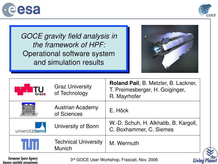
GOCE gravity field analysis in the framework of HPF: Operational software system and simulation results. Roland Pail , B. Metzler, B. Lackner, T. Preimesberger, H. Goiginger, R. Mayrhofer. Graz University of Technology. Austrian Academy of Sciences. E. Höck.

E N D
GOCE gravity field analysis in the framework of HPF: Operational software system and simulation results Roland Pail, B. Metzler, B. Lackner, T. Preimesberger, H. Goiginger,R. Mayrhofer Graz University of Technology Austrian Academy of Sciences E. Höck W.-D. Schuh, H. Alkhatib, B. Kargoll, C. Boxhammer, C. Siemes University of Bonn Technical University Munich M. Wermuth 3rd GOCE User Workshop, Frascati, Nov. 2006
GOCE gravity field analysis in the framework of HPF: Operational software system and simulation results Contents • Software architecture • Product flow, demonstrated on the basis of a realistic numerical case study • Discussion of selected topics (SGG filter, regularization, covariance propagation) • Summary & conclusions 3rd GOCE User Workshop, Frascati, Nov. 2006
SPF6000: Main components • Quick-Look Gravity Field Analysis (QL-GFA) • Fast approximate gravity field solutions • Analysis of SST and SGG input data • in parallel to the mission • latency: 4 hours (QL-A: based on Level 1b data) 2 days (QL-B: intermediate Level 2 data) • common PC • Core Solver (CS) • Rigorous ultimate-precision solution • Final Solver: SST, SGG: full var./covar. matrices • Tuning Machine: - pcgma - Data inspection • Parallel processing on Linux-PC cluster • SST processing: energy integral approach 3rd GOCE User Workshop, Frascati, Nov. 2006
SST NEQ‘s • SGG filters • quality flags • QL gravity field models • GOCE error PSD est. • Quality Report sheets • regularization/ weighting parameters SGG NEQ‘s EGM_QLA_2 EGM_QLB_2i EGM_QLK_2i • Gravity field model • Full variance-covariance matrix EGM_TIM_2i EGM_TVC_2i SPF6000: Architectural Design & Product Flow • Orbits • Gravity gradients INPUT DATA • Attitude information • Auxiliary data CORESOLVER QL-GFA Tuning Machine SST proc. • SST-only solution • SGG-only solution • combined solution • Quality analysis of SGG residuals • pcgma solution • SGG filter design • data inspection • SST-only solution SGG proc. • Assembling of SGG NEQ‘s Solution • Solution of combined system incl. regularization/opt. weighting
SPF6000: HPF Acceptance Review 2*: Test Data Orbit • 60 days, 1 Hz sampling rate • based on EGM96, degree/order 200 • noise: orbit positions: = 3 cm orbit velocities: = 0.1 mm/s • satellite altitude ~240 km • realistic accelerometry Attitude • quaternions describing rotation between inertial (IRF) and gradiometer reference frame (GRF) Gravity gradients • gradients in GRF along orbit, 1 Hz sampled • based on EGM96, degree/order 360 • realistic gradiometer noise assumption Addit. products • Auxiliary data: IERS products, ephemeris, temp.var. corr. • A priori SGG error model (generated from „true“ SGG noise) * HPF Acceptance Review (AR) 2: test of operational HPF system at the end of Development Phase 2
SPF6000: HPF Acceptance Review 2: Test Data (2) Gradiometer error PSD
SPF6000: QL-GFA Quick-Look Gravity Field Analysis
QL-GFA: Gravity field results: QL-A vs. QL-B Coeff.dev. from EGM96 MSE estimates QL-A(Level 1b data) SGG-only solution EGM_QLA_2 QL-B(Level 2 data) combined solution EGM_QLB_2i
mGal mGal -10 -5 0 5 10 -10 -5 0 5 10 QL-GFA: Gravity field results Degree error median with QL-A: SGG-only QL-B: SST-only SGG-only combined SST+SGG Cumulative gravity anomaly errors at D/O 200 SST+SGG SGG-only = 2.9 mGal = 1.8 mGal
QL-GFA: Gradiometer error PSD estimation SGG error PSD estimate EGM_QLK_2i VXX Spectral leakage
SPF 6000: Core Solver Core Solver
SST NEQ‘s • SGG filters • quality flags • QL gravity field models • GOCE error PSD est. • Quality Report sheets • regularization/ weighting parameters SGG NEQ‘s EGM_QLA_2 EGM_QLB_2i EGM_QLK_2i • Gravity field model • Full variance-covariance matrix EGM_TIM_2i EGM_TVC_2i SPF6000: Architectural Design & Product Flow • Orbits • Gravity gradients INPUT DATA • Attitude information • Auxiliary data CORESOLVER QL-GFA Tuning Machine SST proc. • SST-only solution • SGG-only solution • combined solution • Quality analysis of SGG residuals • pcgma solution • SGG filter design • data inspection • SST-only solution SGG proc. • Assembling of SGG NEQ‘s Solution • Solution of combined system incl. regularization/opt. weighting
Core Solver: Tuning Machine Tuning Machine • SGG filter design • data inspection • pcgma solution • stand-alone gravity field solver • optimum regularization &weighting parameters • filters describe the metrics of the normal equation systems • analysis of residuals • outlier detection
Core Solver: Tuning Machine: Filter design # Cascades (xx / yy / zz) Filter effective order (xx / yy / zz) Warmup # positions 0020 (2 / 2 / 2) 40000 52 / 42 / 32 VXX
Core Solver: Final Solver Parallel processing on Linux-PC-cluster(54 Dual-Xeon 2.6GHz PCs, Gigabit-Ethernet connection, performance ~210 GFlops) • SST processing: energy integral • SGG assembling: full normal equations • Solution (Cholesky reduction) EGM_TIM_2i • Inversion full variance-covar. matrix EGM_TVC_2i
Core Solver: Final Solver Assembling of SGG normal equations • parameterization complete up to D/O 204 (see below) • SGG filtering: cascaded filters: filter orders 52 (XX), 42 (YY), 32 (ZZ) Computation of solution (Cholesky reduction and inversion) • Regularization: Spherical Cap regularization, using an independently computed SST-only solution complete to D/O 50 as stabilizing function in the polar cap regions. • (Expected geoid height errors in the polar cap regions mainly due to spectral leakage of the D/O 50 SST solution: ~2 m) • Weighting: Optimum relative weighting factor of SST solution = 1.0 (since SST normal equations are properly scaled) • Spectral leakage: In order to further reduce (small) leakage effects, the normal equations were originally set-up complete to D/O 204, and finally the coefficients an the variance-covariance matrix was truncated at D/O 200. GOCE-only solution in a strict sence, i.e.,NO a priori gravity field information is inherent !!!
96.6° Core Solver: Spherical Cap Regularization Idea:Introducing a stabilizing function at the poles and force the signal toward this function (Metzler & Pail, 2005: Studia geophys. geod.) Advantage:No significant regularization bias in the regions covered by measurements.
Core Solver: Final Solution Coeff.dev. from EGM96 Error estimates Degree error median • Coefficients: EGM_TIM_2i Var.-covar. matrix: EGM_TVC_2i
AR2 (2 months) || < 83° N [cm] 2.93 g [mGal] 0.81 *Numerical case studies (based on longer data sets) revealed that assumption of error decreases with is justified. Core Solver: Final Solution Cumulative geoid height errors Cov. prop. geoid height errors atD/O 200 m m 2 MOPs* (12 months) 1 MOP* (6 months) 1.20 0.33 1.69 0.47
with Special subject: covariance propagation [1] Be aware: GOCE will provide the FULL variance-covariance matrix m
cm cm Special subject: covariance propagation [1] with Covar. prop. geoid heights [cm] full
Special subject: covariance propagation [2] with Geoid height error covariances
Special subject: GOCE performance vs. altitude Relative performance of GOCE mission depending on orbit altitude 300 km 280 km Relative degradation of gravity anomalies 260 km 250 km 240 km 220 km
Summary & conclusions • Sub-Processing Facility (SPF) 6000: software is now fully implemented, and the hardware and software system is integrated. • Successful test in the frame of the HPF Acceptance Review 2. SPF 6000 is ready for operation.
Core Solver: Covariance propagation: Add-on [1] Cumulative geoid height errors Cov. prop. geoid height errors atD/O 200 m m Average geoid height error per latitude