Big Data Mining 巨量資料探勘
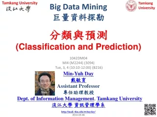
Tamkang University. Tamkang University. 分類與預測 (Classification and Prediction). Big Data Mining 巨量資料探勘. 1042DM04 MI4 (M2244) (3094) Tue, 3, 4 (10:10-12:00) (B216). Min-Yuh Day 戴敏育 Assistant Professor 專任助理教授 Dept. of Information Management , Tamkang University 淡江大學 資訊管理學系

Big Data Mining 巨量資料探勘
E N D
Presentation Transcript
Tamkang University Tamkang University 分類與預測 (Classification and Prediction) Big Data Mining巨量資料探勘 1042DM04 MI4 (M2244) (3094) Tue, 3, 4 (10:10-12:00) (B216) Min-Yuh Day 戴敏育 Assistant Professor 專任助理教授 Dept. of Information Management, Tamkang University 淡江大學資訊管理學系 http://mail. tku.edu.tw/myday/ 2016-03-08
課程大綱 (Syllabus) 週次 (Week) 日期 (Date) 內容 (Subject/Topics) 1 2016/02/16 巨量資料探勘課程介紹 (Course Orientation for Big Data Mining) 2 2016/02/23 巨量資料基礎:MapReduce典範、Hadoop與Spark生態系統 (Fundamental Big Data: MapReduce Paradigm, Hadoop and Spark Ecosystem) 3 2016/03/01 關連分析 (Association Analysis) 4 2016/03/08 分類與預測 (Classification and Prediction) 5 2016/03/15 分群分析 (Cluster Analysis) 6 2016/03/22 個案分析與實作一 (SAS EM 分群分析): Case Study 1 (Cluster Analysis – K-Means using SAS EM) 7 2016/03/29 個案分析與實作二 (SAS EM 關連分析): Case Study 2 (Association Analysis using SAS EM)
課程大綱 (Syllabus) 週次 (Week) 日期 (Date) 內容 (Subject/Topics) 8 2016/04/05 教學行政觀摩日 (Off-campus study) 9 2016/04/12 期中報告 (Midterm Project Presentation) 10 2016/04/19 期中考試週 (Midterm Exam) 11 2016/04/26 個案分析與實作三 (SAS EM 決策樹、模型評估):Case Study 3 (Decision Tree, Model Evaluation using SAS EM) 12 2016/05/03 個案分析與實作四 (SAS EM 迴歸分析、類神經網路): Case Study 4 (Regression Analysis, Artificial Neural Network using SAS EM) 13 2016/05/10 Google TensorFlow 深度學習 (Deep Learning with Google TensorFlow) 14 2016/05/17 期末報告 (Final Project Presentation) 15 2016/05/24 畢業班考試 (Final Exam)
Outline • Classification and Prediction • Supervised Learning (Classification) • Decision Tree (DT) • Information Gain (IG) • Support Vector Machine (SVM) • Data Mining Evaluation • Accuracy • Precision • Recall • F1 score (F-measure) (F-score)
A Taxonomy for Data Mining Tasks Source: Turban et al. (2011), Decision Support and Business Intelligence Systems
What is the class (buys_computer = “yes” or buys_computer = “no”) for a customer (age=youth, income=medium, student =yes, credit= fair )?
What is the class (buys_computer = “yes” or buys_computer = “no”) for a customer (age=youth, income=medium, student =yes, credit= fair )? Yes = 0.0889 No = 0.0167
Classification vs. Prediction • Classification • predicts categorical class labels (discrete or nominal) • classifies data (constructs a model) based on the training set and the values (class labels) in a classifying attribute and uses it in classifying new data • Prediction • models continuous-valued functions • i.e., predicts unknown or missing values • Typical applications • Credit approval • Target marketing • Medical diagnosis • Fraud detection Source: Han & Kamber (2006)
Data Mining Methods: Classification Most frequently used DM method Part of the machine-learning family Employ supervised learning Learn from past data, classify new data The output variable is categorical (nominal or ordinal) in nature Classification versus regression? Classification versus clustering? Source: Turban et al. (2011), Decision Support and Business Intelligence Systems
Classification Techniques Decision Tree analysis (DT) Statistical analysis Neural networks (NN) Deep Learning (DL) Support Vector Machines (SVM) Case-based reasoning Bayesian classifiers Genetic algorithms (GA) Rough sets Source: Turban et al. (2011), Decision Support and Business Intelligence Systems
Example of Classification • Loan Application Data • Which loan applicants are “safe” and which are “risky” for the bank? • “Safe” or “risky” for load application data • Marketing Data • Whether a customer with a given profile will buy a new computer? • “yes” or “no” for marketing data • Classification • Data analysis task • A model or Classifier is constructed to predict categorical labels • Labels: “safe” or “risky”; “yes” or “no”; “treatment A”, “treatment B”, “treatment C” Source: Han & Kamber (2006)
What Is Prediction? • (Numerical) prediction is similar to classification • construct a model • use model to predict continuous or ordered value for a given input • Prediction is different from classification • Classification refers to predict categorical class label • Prediction models continuous-valued functions • Major method for prediction: regression • model the relationship between one or more independent or predictor variables and a dependent or response variable • Regression analysis • Linear and multiple regression • Non-linear regression • Other regression methods: generalized linear model, Poisson regression, log-linear models, regression trees Source: Han & Kamber (2006)
Linear Regression Nonlinear Regression Other Regression Methods Prediction Methods Source: Han & Kamber (2006)
Classification and Prediction • Classification and prediction are two forms of data analysis that can be used to extract models describing important data classes or to predict future data trends. • Classification • Effective and scalable methods have been developed for decision trees induction, Naive Bayesian classification, Bayesian belief network, rule-based classifier, Backpropagation, Support Vector Machine (SVM), associative classification, nearest neighbor classifiers, and case-based reasoning, and other classification methods such as genetic algorithms, rough set and fuzzy set approaches. • Prediction • Linear, nonlinear, and generalized linear models of regression can be used for prediction. Many nonlinear problems can be converted to linear problems by performing transformations on the predictor variables. Regression trees and model trees are also used for prediction. Source: Han & Kamber (2006)
Classification—A Two-Step Process • Model construction: describing a set of predetermined classes • Each tuple/sample is assumed to belong to a predefined class, as determined by the class label attribute • The set of tuples used for model construction is training set • The model is represented as classification rules, decision trees, or mathematical formulae • Model usage: for classifying future or unknown objects • Estimate accuracy of the model • The known label of test sample is compared with the classified result from the model • Accuracy rate is the percentage of test set samples that are correctly classified by the model • Test set is independent of training set, otherwise over-fitting will occur • If the accuracy is acceptable, use the model to classify data tuples whose class labels are not known Source: Han & Kamber (2006)
Supervised Learning vs. Unsupervised Learning • Supervised learning (classification) • Supervision: The training data (observations, measurements, etc.) are accompanied by labels indicating the class of the observations • New data is classified based on the training set • Unsupervised learning(clustering) • The class labels of training data is unknown • Given a set of measurements, observations, etc. with the aim of establishing the existence of classes or clusters in the data Source: Han & Kamber (2006)
Issues Regarding Classification and Prediction: Data Preparation • Data cleaning • Preprocess data in order to reduce noise and handle missing values • Relevance analysis (feature selection) • Remove the irrelevant or redundant attributes • Attribute subset selection • Feature Selection in machine learning • Data transformation • Generalize and/or normalize data • Example • Income: low, medium, high Source: Han & Kamber (2006)
Issues: Evaluating Classification and Prediction Methods • Accuracy • classifier accuracy: predicting class label • predictor accuracy: guessing value of predicted attributes • estimation techniques: cross-validation and bootstrapping • Speed • time to construct the model (training time) • time to use the model (classification/prediction time) • Robustness • handling noise and missing values • Scalability • ability to construct the classifier or predictor efficiently given large amounts of data • Interpretability • understanding and insight provided by the model Source: Han & Kamber (2006)
Data Classification Process 1: Learning (Training) Step (a) Learning: Training data are analyzed by classification algorithm y= f(X) Source: Han & Kamber (2006)
Data Classification Process 2 (b) Classification: Test data are used to estimate the accuracy of the classification rules. Source: Han & Kamber (2006)
Training Data Classifier (Model) Process (1): Model Construction Classification Algorithms IF rank = ‘professor’ OR years > 6 THEN tenured = ‘yes’ Source: Han & Kamber (2006)
Classifier Testing Data Unseen Data Process (2): Using the Model in Prediction (Jeff, Professor, 4) Tenured? Source: Han & Kamber (2006)
Decision Trees A general algorithm for decision tree building • Employs the divide and conquer method • Recursively divides a training set until each division consists of examples from one class • Create a root node and assign all of the training data to it • Select the best splitting attribute • Add a branch to the root node for each value of the split. Split the data into mutually exclusive subsets along the lines of the specific split • Repeat the steps 2 and 3 for each and every leaf node until the stopping criteria is reached Source: Turban et al. (2011), Decision Support and Business Intelligence Systems
Decision Trees • DT algorithms mainly differ on • Splitting criteria • Which variable to split first? • What values to use to split? • How many splits to form for each node? • Stopping criteria • When to stop building the tree • Pruning (generalization method) • Pre-pruning versus post-pruning • Most popular DT algorithms include • ID3, C4.5, C5; CART; CHAID; M5 Source: Turban et al. (2011), Decision Support and Business Intelligence Systems
Decision Trees • Alternative splitting criteria • Gini index determines the purity of a specific class as a result of a decision to branch along a particular attribute/value • Used in CART • Information gain uses entropy to measure the extent of uncertainty or randomness of a particular attribute/value split • Used in ID3, C4.5, C5 • Chi-square statistics (used in CHAID) Source: Turban et al. (2011), Decision Support and Business Intelligence Systems
Classification by Decision Tree InductionTraining Dataset This follows an example of Quinlan’s ID3 (Playing Tennis) Source: Han & Kamber (2006)
Classification by Decision Tree Induction age? senior >40 middle_aged31..40 youth<=30 student? credit rating? fair excellent no yes Output: A Decision Tree for “buys_computer” yes yes no yes no buys_computer=“yes” or buys_computer=“no” Source: Han & Kamber (2006)
Three possibilities for partitioning tuples based on the splitting Criterion Source: Han & Kamber (2006)
Algorithm for Decision Tree Induction • Basic algorithm (a greedy algorithm) • Tree is constructed in a top-down recursive divide-and-conquer manner • At start, all the training examples are at the root • Attributes are categorical (if continuous-valued, they are discretized in advance) • Examples are partitioned recursively based on selected attributes • Test attributes are selected on the basis of a heuristic or statistical measure (e.g., information gain) • Conditions for stopping partitioning • All samples for a given node belong to the same class • There are no remaining attributes for further partitioning – majority voting is employed for classifying the leaf • There are no samples left Source: Han & Kamber (2006)
Attribute Selection Measure • Notation: Let D, the data partition, be a training set of class-labeled tuples. Suppose the class label attribute has m distinct values defining m distinct classes, Ci (for i = 1, … , m). Let Ci,D be the set of tuples of class Ci in D. Let |D| and | Ci,D | denote the number of tuples in D and Ci,D , respectively. • Example: • Class: buys_computer= “yes” or “no” • Two distinct classes (m=2) • Class Ci (i=1,2): C1 = “yes”,C2 = “no” Source: Han & Kamber (2006)
Attribute Selection Measure: Information Gain (ID3/C4.5) • Select the attribute with the highest information gain • Let pi be the probability that an arbitrary tuple in D belongs to class Ci, estimated by |Ci, D|/|D| • Expected information (entropy) needed to classify a tuple in D: • Information needed (after using A to split D into v partitions) to classify D: • Information gained by branching on attribute A Source: Han & Kamber (2006)
log2 (1) = 0 log2 (2) = 1 log2 (3) = 1.5850 log2 (4) = 2 log2 (5) = 2.3219 log2 (6) = 2.5850 log2 (7) = 2.8074 log2 (8) = 3 log2 (9) = 3.1699 log2 (10) = 3.3219 log2 (0.1) = -3.3219 log2 (0.2) = -2.3219 log2 (0.3) = -1.7370 log2 (0.4) = -1.3219 log2 (0.5) = -1 log2 (0.6) = -0.7370 log2 (0.7) = -0.5146 log2 (0.8) = -0.3219 log2 (0.9) = -0.1520 log2 (1) = 0
Class-labeled training tuples from the AllElectronics customer database The attribute age has the highest information gain and therefore becomes the splitting attribute at the root node of the decision tree Source: Han & Kamber (2006)
Class P: buys_computer = “yes” Class N: buys_computer = “no” means “age <=30” has 5 out of 14 samples, with 2 yes’es and 3 no’s. Hence Similarly, Attribute Selection: Information Gain Source: Han & Kamber (2006)
What is the class (buys_computer = “yes” or buys_computer = “no”) for a customer (age=youth, income=medium, student =yes, credit= fair )?
What is the class (buys_computer = “yes” or buys_computer = “no”) for a customer (age=youth, income=medium, student =yes, credit= fair )? Yes = 0.0889 No = 0.0167
Table 1 shows the class-labeled training tuples from customer database. Please calculate and illustrate the final decision tree returned by decision tree induction using information gain. (1) What is the Information Gain of “age”? (2) What is the Information Gain of “income”? (3) What is the Information Gain of “student”? (4) What is the Information Gain of “credit_rating”? (5) What is the class (buys_computer = “yes” or buys_computer = “no”) for a customer (age=youth, income=medium, student =yes, credit= fair ) based on the classification result by decision three induction?
Attribute Selection Measure: Information Gain (ID3/C4.5) • Select the attribute with the highest information gain • Let pi be the probability that an arbitrary tuple in D belongs to class Ci, estimated by |Ci, D|/|D| • Expected information (entropy) needed to classify a tuple in D: • Information needed (after using A to split D into v partitions) to classify D: • Information gained by branching on attribute A Source: Han & Kamber (2006)
log2 (1) = 0 log2 (2) = 1 log2 (3) = 1.5850 log2 (4) = 2 log2 (5) = 2.3219 log2 (6) = 2.5850 log2 (7) = 2.8074 log2 (8) = 3 log2 (9) = 3.1699 log2 (10) = 3.3219 log2 (0.1) = -3.3219 log2 (0.2) = -2.3219 log2 (0.3) = -1.7370 log2 (0.4) = -1.3219 log2 (0.5) = -1 log2 (0.6) = -0.7370 log2 (0.7) = -0.5146 log2 (0.8) = -0.3219 log2 (0.9) = -0.1520 log2 (1) = 0
Class P (Positive): buys_computer = “yes” Class N (Negative): buys_computer = “no” P(buys = yes) = Pi=1 = P1= 6/10 = 0.6 P(buys = no) = Pi=2 = P2= 4/10 = 0.4 log2 (1) = 0 log2 (2) = 1 log2 (3) = 1.5850 log2 (4) = 2 log2 (5) = 2.3219 log2 (6) = 2.5850 log2 (7) = 2.8074 log2 (8) = 3 log2 (9) = 3.1699 log2 (10) = 3.3219 log2 (0.1) = -3.3219 log2 (0.2) = -2.3219 log2 (0.3) = -1.7370 log2 (0.4) = -1.3219 log2 (0.5) = -1 log2 (0.6) = -0.7370 log2 (0.7) = -0.5146 log2 (0.8) = -0.3219 log2 (0.9) = -0.1520 log2 (1) = 0 Step 1: Expected information Info(D) = I(6,4) = 0.971
Step 2: Information Step 3: Information Gain Info(D) = I(6,4) = 0.971 (1) Gain(age)= 0.3221
Info(D) = I(6,4) = 0.971 (2) Gain(income)= 0.02

