Download
1 / 14
140 likes | 245 Vues
Learn about effective techniques like radial velocity, transit photometry, and microlensing for detecting exoplanets, with examples such as Neptune-mass planets and microlensing planets. Understand how to determine orbital parameters, estimate orbital periods, and refine orbital solutions. Discover the pulsar planet story and explore timing residuals to unravel the latest puzzles. Find out how Vr time series are constructed and examine examples of orbital solutions under construction. Gain insights into future challenges and advancements in astrometry and planet imaging.

E N D
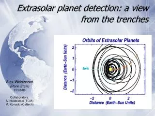
Extrasolar planet detection: a view from the trenches Alex Wolszczan (Penn State) 01/23/06 Collaborators: A. Niedzielski (TCfA) M. Konacki (Caltech)
Methods that actually work … Radial velocity Pulse timing Microlensing Transit photometry
Some examples… Neptune-mass planet The transit classic: HD209458 Microlensing planet A “super-comet” around PSR B1257+12?
Orbits from Vr measurements • Observations are given in the form of a time series, Vr(i), at epochs t(i), i = 1,…,n • A transition from t(i) to (i) is accomplished in two steps: Equation for eccentric anomaly, E • From the fit (least squares, etc.), one determines parameters K, e, , T, P
…and from pulsar timing • In phase-connected timing, one models pulse phase in terms of spin frequency and its derivatives and tries to keep pulse count starting at t0 • A predicted time-of-arrival (TOA) of a pulse at the Solar System barycenter depends on a number of factors:
Determining binary orbits… • Collect data: measure Vr’s, TOA’s, P’s • Estimate orbital period, Pb (see below) • Use Vr’s to estimate a1sini, e, T0, Pb, (use P’s to obtain an “incoherent orbital solution”) • Use TOA’s to derive a “phase-connected” orbital solution
Figuring out the orbital period… • Go Lomb-Scargle! If in doubt, try this procedure (borrowed from Joe Taylor): • Get the best and most complete time series of your observable (the hardest part) • Define the shortest reasonable Pb for your data set • Compute orbital phases, I = mod(ti/Pb,1.0) • Sort (Pi, ti, I) in order of increasing • Compute s2 = ∑(Pj-Pj-1)2 ignoring terms for which j- j-1> 0.1 • Increment Pb = [1/Pb-0.1/(tmax-tmin)]-1 • Repeat these steps until an “acceptable” Pb has been reached • Choose Pb for the smallest value of s2
… and the latest puzzle to play with • Timing (TOA) residuals at 430 MHz show a 3.7-yr periodicity with a ~10 µs amplitude • At 1400 MHz, this periodicity has become evident in late 2003, with a ~2 µs amplitude • Two-frequency timing can be used to calculate line-of-sight electron column density (DM) variations, using the cold plasma dispersion law. The data show a typical long-term, interstellar trend in DM, with the superimposed low-amplitude variations • By definition, these variations perfectly correlate with the timing residual variations in (a) Because a dispersive delay scales as 2, the observed periodic TOA variations are most likely a superposition of a variable propagation delay and the effect of a Keplerian motion of a very low-mass body
One of the promising candidates… • Periods from time domain search: 118, 355 days • Periods from periodogram: 120, 400 days • Periods from simplex search: 118, 340, also 450 days
…and the best orbital solutions • P~340 (e~0.35) appears to be best (lowest rms residual, 2 ~ 1) • This case will probably be resolved in the next 2 months, after >2 years of observations
Summary… • Given: a time series of your observable • Sought: a stable orbital solution to get orbital parameters and planet characteristics • Question: astrophysical viability of the model (e.g. stellar activity, neutron star seismology, fake transit events by background stars) • Future: new challenges with the advent of high-precision astrometry from ground and space and planet imaging in more distant future