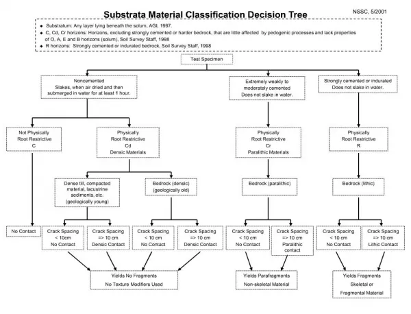
Decision Tree Classification

1. Decision Tree Classification Tomi Yiu CS 632 — Advanced Database Systems April 5, 2001

2. Papers • Manish Mehta, Rakesh Agrawal, Jorma Rissanen: SLIQ: A Fast Scalable Classifier for Data Mining. • John C. Shafer, Rakesh Agrawal, Manish Mehta: SPRINT: A Scalable Parallel Classifier for Data Mining. • Pedro Domingos, Geoff Hulten: Mining high-speed data streams.

3. Outline • Classification problem • General decision tree model • Decision tree classifiers • SLIQ • SPRINT • VFDT (Hoeffding Tree Algorithm)

4. Classification Problem • Given a set of example records • Each record consists of • A set of attributes • A class label • Build an accurate model for each class based on the set of attributes • Use the model to classify future data for which the class labels are unknown

5. A Training set

6. Classification Models • Neural networks • Statistical models – linear/quadratic discriminants • Decision trees • Genetic models

7. Why Decision Tree Model? • Relatively fast compared to other classification models • Obtain similar and sometimes better accuracy compared to other models • Simple and easy to understand • Can be converted into simple and easy to understand classification rules

8. A Decision Tree Age < 25 Car Type in {sports} High High Low

9. Decision Tree Classification • A decision tree is created in two phases: • Tree Building Phase • Repeatedly partition the training data until all the examples in each partition belong to one class or the partition is sufficiently small • Tree Pruning Phase • Remove dependency on statistical noise or variation that may be particular only to the training set

10. Tree Building Phase • General tree-growth algorithm (binary tree) Partition(Data S) If (all points in S are of the same class) then return; for each attribute A do evaluate splits on attribute A; Use best split to partition S into S1 and S2; Partition(S1); Partition(S2);

11. Tree Building Phase (cont.) • The form of the split depends on the type of the attribute • Splits for numeric attributes are of the form A  v, where v is a real number • Splits for categorical attributes are of the form A  S’, where S’ is a subset of all possible values of A

12. Splitting Index • Alternative splits for an attribute are compared using a splitting index • Examples of splitting index: • Entropy ( entropy(T) = - pj x log2(pj) ) • Gini Index ( gini(T) = 1 - pj2 ) (pj is the relative frequency of class j in T)

13. The Best Split • Suppose the splitting index is I(), and a split partitions S into S1 and S2 • The best split is the split that maximizes the following value: I(S) - |S1|/|S| x I(S1) + |S2|/|S| x I(S2)

14. Tree Pruning Phase • Examine the initial tree built • Choose the subtree with the least estimated error rate • Two approaches for error estimation: • Use the original training dataset (e.g. cross –validation) • Use an independent dataset

15. SLIQ - Overview • Capable of classifying disk-resident datasets • Scalable for large datasets • Use pre-sorting technique to reduce the cost of evaluating numeric attributes • Use a breath-first tree growing strategy • Use an inexpensive tree-pruning algorithm based on the Minimum Description Length (MDL) principle

16. Data Structure • A list (class list) for the class label • Each entry has two fields: the class label and a reference to a leaf node of the decision tree • Memory-resident • A list for each attribute • Each entry has two fields: the attribute value, an index into the class list • Written to disk if necessary

17. An illustration of the Data Structure

18. Pre-sorting • Sorting of data is required to find the split for numeric attributes • Previous algorithms sort data at every node in the tree • Using the separate list data structure, SLIQ only sort data once at the beginning of the tree building phase

19. After Pre-sorting

20. Node Split • SLIQ uses a breath-first tree growing strategy • In one pass over the data, splits for all the leaves of the current tree can be evaluated • SLIQ uses gini-splitting index to evaluate split • Frequency distribution of class values in data partitions is required

21. Class Histogram • A class histogram is used to keep the frequency distribution of class values for each attribute in each leaf node • For numeric attributes, the class histogram is a list of <class, frequency> • For categorical attributes, the class histogram is a list of <attribute value, class, frequency>

22. Evaluate Split for each attribute A traverse attribute list of A for each value v in the attribute list find the corresponding class and leaf node update the class histogram in the leaf l if A is a numeric attribute then compute splitting index for test (Av) for leaf l if A is a categorical attribute then for each leaf of the tree do find subset of A with the best split

23. Subsetting for Categorical Attributes If cardinality of S is less than a threshold all of the subsets of S are evaluated else start an empty subset S’ repeat adds the element of S to S’ which gives the best split until there is no improvement

24. Partition the data • Partition can be done by updating the leaf reference of each entry in the class list • Algorithm: for each attribute A used in a split traverse attribute list of A for each value v in the list find corresponding class label and leaf l find the new node, n, to which v belongs by applying the splitting test at l update the leaf reference to n

25. Example of Evaluating Splits Initial Histogram Evaluate split (age  17) Evaluate split (age  32)

26. Example of Updating Class List Age  23 N1 N2 N3 N3 (New value)

27. MDL Principle • Given a model, M, and the data, D • MDL principle states that the best model for encoding data is the one that minimizes Cost(M,D) = Cost(D|M) + Cost(M) • Cost (D|M) is the cost, in number of bits, of encoding the data given a model M • Cost (M) is the cost of encoding the model M

28. MDL Pruning Algorithm • The models are the set of trees obtained by pruning the initial decision T • The data is the training set S • The goal is to find the subtree of T that best describes the training set S (i.e. with the minimum cost) • The algorithm evaluates the cost at each decision tree node to determine whether to convert the node into a leaf, prune the left or the right child, or leave the node intact.

29. Encoding Scheme • Cost(S|T) is defined as the sum of all classification errors • Cost(M) includes • The cost of describing the tree • number of bits used to encode each node • The costs of describing the splits • For numeric attributes, the cost is 1 bit • For categorical Attributes, the cost is ln(nA), where nA is the total number of tests of the form A  S’ used

30. Performance (Scalability)

31. SPRINT - Overview • A fast, scalable classifier • Use pre-sorting method as in SLIQ • No memory restriction • Easily parallelized • Allow many processors to work together to build a single consistent model • The parallel version is also scalable

32. Data Structure – Attribute List • Each attribute has an attribute list • Each entry of a list has three fields: the attribute value, the class label, and the rid of the record from which these values were obtained • The initial lists are associated with the root • As the node split, the lists will be partitioned and associated with the children • Numeric attributes will be sorted once created • Written to disk if necessary

33. An Example of Attribute Lists

34. Attribute Lists after Splitting

35. Data Structure - Histogram • SPRINT uses gini-splitting index • Histograms are used to capture the class distribution of the attribute records at each node • Two histograms for numeric attributes • Cbelow – maintain data that has been processed • Cabove – maintain data that hasn’t been processed • One histogram for categorical attributes, called count matrix

36. Finding Split Points • Similar to SLIQ except each node has its own attribute lists • Numeric attributes • Cbelow initials to zeros • Cabove initials with the class distribution at that node • Scan the attribute list to find the best split • Categorical attributes • Scan the attribute list to build the count matrix • Use the subsetting algorithm in SLIQ to find the best split

37. Evaluate numeric attributes

38. Evaluate categorical attributes Attribute List Count Matrix

39. Performing the Split • Each attribute list will be partitioned into two lists, one for each child • Splitting attribute • Scan the attribute list, apply the split test, and move records to one of the two new lists • Non-splitting attribute • Cannot apply the split test on non-splitting attributes • Use rid to split attribute lists

40. Performing the Split (cont.) • When partitioning the attribute list of the splitting attribute, insert the rid of each record into a hash table, noting to which child it was moved • Scan the non-splitting attribute lists • For each record, probe the hash table with the rid to find out which child the record should move to • Problem: What should we do if the hash table is too large for the memory?

41. Performing the Split (cont.) • Use the following algorithm to partition the attribute lists if the hash table is too big: Repeat The attribute list of the splitting attribute list is partitioned up to the record for which the hash table will fit in the memory Scan the attribute list of non-splitting attributes to partition the records whose rids are in the hash table Until all the records have been partitioned

42. Parallelizing Classification • SPRINT was designed for parallel classification • Fast and scalable • Similar to the serial version of SPRINT • Each processor has a portion (same size as others) of each attribute lists • For numeric attribute, sort the attributes and partition it into contiguous sorted sections • For categorical attribute, no processing is required and simply partition it based on rid

43. Parallel Data Placement Process 0 Process 1

44. Finding Split Points • For numeric attribute • Each processor has a contiguous section of the list • Initialize Cbelow and Cabove to reflect that some data are in the other processors • Each processor scans its list to find its best split • Processors communicate to determine the best split • For categorical attribute • Each processor builds the count matrix • A coordinator collect all the count matrices • Sum up all counts and find the best split

45. Example of Histograms in Parallel Classification Process 0 Process 1

46. Performing the Splits • Almost identical to the serial version • Except the processor needs <rids, child> information from other processors • After getting information about all rids from other processors, it can build a hash table and partition the attribute lists

47. SLIQ vs. SPRINT • SLIQ has a faster response time • SPRINT can handle larger datasets

48. Data Streams • Data arrive continuously (it’s possible that they come in very fast) • Data size is extremely large, potentially infinite • Couldn’t possibly store all the data

49. Issues • Disk/Memory-resident algorithms require the data to be in the disk/memory • They may need to scan the data multiple times • Need algorithms that read data only once, and only require a small amount of time to process it • Incremental learning method

50. Incremental learning methods • Previous incremental learning methods • Some are efficient, but do not produce accurate model • Some produce accurate model, but very inefficient • Algorithm that is efficient and produces accurate model • Hoeffding Tree Algorithm