Download

1 / 12
140 likes | 284 Vues
Tracking the origin of the seismic noise. Tracking the origin of the seismic noise. Tracking the origin of the seismic noise. Apparent origin of the noise. Average sea wave height. winter. summer. Importance of scattering: a simple laboratory experiment with a few sources. C(A,X).

E N D
Apparent origin of the noise Average sea wave height winter summer
Importance of scattering: a simple laboratory experiment with a few sources C(A,X) Correlations in water G(A,X) travel time A Xs sources receivers Correlations in presence of scattering
x3 x θ y n x1 ψ THE 2D SCALAR CASE H(2)n(kr)=Jn(kr) − iYn(kr) Illumination by plane waves Azimuthal average over ψ leads to SPAC method k C
Keiiti Aki x3 x θ y n x1 ψ A isotropic distribution of plane waves in an homogeneous body : the local approach THE 2D SCALAR CASE SH waves in a homogeneous elastic medium Propagation takes place in the x1-x3 plane. Therefore, the antiplane (out-of-plane) displacement v(x,t) fulfils the wave equation where β = shear wave velocity and t = time. A typical harmonic, homogeneous plane wave can be written as where, F(ω, ψ) = complex waveform, ω=circular frequency, xT = (x1, x3) = Cartesian coordinates x1= r cosθ = , x3 = r sinθ = , with r,θ = polar coordinates nj = direction cosines (n1= cos ψ , n3 = sin ψ ) Consider the auto-correlation of the motion, evaluated at positions x and y, respectively. For simplicity assume y at the origin: .
Cross-correlations of seismic noise: ANMO - CCM (from Shapiro and Campillo, GRL, 2004) 30 days of vertical motion Dispersion analysis global model by Ritzwoller et al. 2002
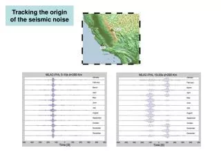
correlations computed over four different three-week periods PHL - MLAC 290 km band- passed 15 - 30 s band- passed 5 - 10 s repetitive measurements provide uncertainty estimations
t G/2 (Re) (Im, Re) t (Im) Causality