Chapter 2 Utility and Choice
Chapter 2 Utility and Choice. Objective. Build a model to understand how a consumer makes decisions under scarcity. To understand his choice we need to know: Preferences Constraints. Utility. Consumer makes a choice that results in the maximum satisfaction or UTILITY.

Chapter 2 Utility and Choice
E N D
Presentation Transcript
Objective • Build a model to understand how a consumer makes decisions under scarcity. • To understand his choice we need to know: • Preferences • Constraints
Utility • Consumer makes a choice that results in the maximum satisfaction or UTILITY. • Two goods available: X1 and X2. • Utility = U(X1, X2; other things) • Utility depends on the amount of X1 and X2 consumed and other things. • Assume other things are held constant.
Three Assumptions About Preferences We make the following assumptions about preference so we can represent preferences by a utility function • Completeness • Given two options, A and B, a person can state which option they prefer or whether they find both options equally attractive. • Transitivity • Preferences are internally consistent. • If I prefer A to B, and prefer B to C, then I must prefer A to C. • More is Better • Economic “goods” • What’s an economic “bad”?
More is Better Graphically Combinations of X and Y in the green area are preferred to (X*, Y*) Quantity of Y per week (X*, Y*) is preferred to combinations of X an Y in the red area. Can’t say about the other points. ? Y* ? Quantity of X per week X*
Indifference Curves • We want to find a way to compare points in the two ? regions from the last picture. • Two goods: soft drinks and hamburgers. • Indifference curve • A curve that shows all the combinations of two goods that give the same level of utility • If you get the same utility you must be indifferent.
Indifference Curve Let’s say you are indifferent between A, B, C and D. Hamburgers per week Draw a curve through those points. Every point gives the same level of utility. A 6 B 4 C 3 D 2 U1 Soft drinks per week 6 2 3 4 5
Indifference Curve What can we say about combination E? Hamburgers per week What about F? A 6 B E 4 C 3 D 2 U1 F Soft drinks per week 6 2 3 4 5
Indifference Curve Why does the indifference curve have a negative slope? Hamburgers per week Because, if you give up hamburgers, you need to get more soft drinks to still get the same level of utility. A 6 B E 4 C 3 D 2 U1 F Soft drinks per week 6 2 3 4 5
Indifference Curve Maps An indifference curve map shows the utility a person gets from all possible combinations of two goods. Hamburgers per week As you move to the northwest, utility increases: U3 > U2 > U1 U3 U2 U1 Soft drinks per week
Marginal Rate of Substitution (MRS) • The absolute value of the slope of the indifference curve • The MRS measures the rate at which you are willing to reduce the consumption of one good to get one more unit of another good and still remain indifferent.
MRS From A to B: the person is willing to give up 2 burgers to get 1 more soda. From B to C: the person is willing to give up 1 burger to get 1 more soda. Hamburgers per week From C to D: the person is willing to give up ½ burger to get 1 more soda. A 6 B E 4 C 3 D 2 U1 F Soft drinks per week 6 2 3 4 5
Diminishing MRS • As you consume more and more soda, the number of burgers you are willing to give up to get one more soda gets smaller and smaller. • This is known as diminishing marginal rate of substitution. • People prefer balanced consumption to extremes. • From convexity • Move along the indifference curve • Same utility level • MRS decreases
Calculating MRS • MRS=-MU1/MU2 • Calculate Mui, where i =1 or 2, from utility function
Convexity of Preferences Suppose we create a basket that is ½ of A and ½ of D: point G. Hamburgers per week You would prefer 4 burgers and 4 sodas to 6 of one good and 2 of the other good. A 6 G 4 D 2 U1 Soft drinks per week 4 0 2 3 6
Upward sloping indifference curves • A good and a bad • Flat indifference curves • Goods that yield no utility • Useless goods • Straight-line indifference curves • Goods that are perfect substitutes • MRS - constant along an indifference curve • In a two-good world • Indifference curve - straight line Representing Preferences Graphically
(b) (a) Good 2 (x 2) Good 2 (x 2) 10 9 5 a 4 -∆x1 -∆x1 +∆x2 0 3 8 11 Good 1 (x 1) 0 Good 1 (x 1) +∆x2 (a) Flat indifference curves. The good measured on the horizontal axis is yielding no utility for the consumer. (b) Straight-line indifference curves: perfect substitutes. The same amount of good 2 is always needed to compensate the consumer for the loss of one unit of good 1.
Right-angle indifference curves • Goods that are perfect complements • Must be consumed in a fixed ratio to produce utility • Bowed-out indifference curves • Nonconvex preferences Representing Preferences Graphically
(d) (c) Good 2 (x 2) Good 2 (x 2) +∆x2 +∆x2 -∆x1 +∆x2 -∆x1 11 I1 -∆x1 10 c b a b a 0 5 6 Good 1 (x 1) 0 Good 1 (x 1) (c) Right-angle indifference curves: perfect complements. Adding any amount of only one good to bundle a yields no additional utility. (d) Bowed-out indifference curves: non-convex preferences and the MRS. As the consumer getsmore of good 2, he values it more.
Perfect substitutes Pepsi 0 Coke Mary’s marginal rate of substitution is constant at any bundle of Pepsi and Coke.
Budget line Good 2 150 100 50 Good 1 0 50 100 150 Points on the budget line indicate all the bundles of goods that the consumer can afford.
Budget Line and Government Policy What is the effect of the following on the budget line? • Quantity tax • Value tax • Lump sum tax • Voucher • rationing
Optimal consumption bundle • Maximize consumer’s utility • Within the economically feasible set • Best bundle • According to consumer’s preferences • Characteristics of optimal bundles • Indifference curve tangent to budget line • Slope of indifference curve = MRS = -∆x2/∆x1 • Slope of budget line = price ratio = p1/p2 • MRS = p1/p2 Optimal Consumption Bundle
The optimal consumption bundle Good 2 (x 2) B +1 -3 -4 +1 k e m n x z 0 Good 1 (x 1) F B’ At the optimal point e, the indifference curve is tangent to the budget line