Cataclysmic Variables

Cataclysmic Variables Mark Cropper Mullard Space Science Laboratory University College London

Course Structure • Brief historical introduction and context • Types and classes. • Non-magnetic systems • Magnetic systems: Polars and Intermediate Polars • Short and ultra-short period systems • Formation, evolution • The role of CVs within the larger scheme of astrophysical studies.

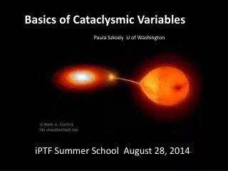
Cataclysmic Variables: what are they?

2 CVs: what are they? • Cataclysmic Variables are • semi-detached binaries accreting • from a red dwarf main-sequence-like secondary star • to a more massive white dwarf primary star • Roche potential: the gravitational potential around two orbiting point masses – resultant force on a test mass: Centre of Mass credit: csep10.phys.utk.edu

2 Roche Lobe Overflow • Semi-detached secondary star fills its Roche lobe so that it is distorted into a pear shape. • At Lagrangian 1 (L1) point, gravitational and centrifugal forces cancel and material is lost from the secondary star into the primary Roche lobe. • Material falls towards the white dwarf in a stream • The 4 other stationary pointsL2 – L5 are important for orbit theory credit: csep10.phys.utk.edu credit: www.genesismission.org

CVs: main types non-magnetic Intermediate Polar Polar

CVs: Role of the Magnetic Field (1) • magnetic field on primary <106 G (100T)  non-magnetic CV • accretion takes place through a disk • via boundary layeron white dwarf

CVs: Role of the Magnetic Field (2) • magnetic field > 107 G (1000 T) polar/AM Her system • NO DISK: accretion takes place via a stream and accretion column directly onto white dwarf • the magnetic field controls the flow fromsome threading region

CVs: Role of the Magnetic Field (3) • magnetic field ~106 G intermediate polar/DQ Her system • accretion takes place through a hollowed-out disk and then via accretion columns onto the white dwarf • magnetic field controls the flow in the final stages

byHevelius CVs: Some background • First European observation of a CV, Nova Vulpecula, were made in 1670 by a monk Pére Dom Anthelme (2nd magnitude) • Another nova, Nova Oph 1848 discovered by John Russell Hind • The first Dwarf Nova, U Gem, also discovered by J. R. Hind in 1855: noted that it was blue – most unusual for variable stars (mv~13.5); substantial body of observations accrued and early harmonic analyses (Whittaker 1911) • Next Dwarf Nova to be discovered was SS Cyg, in 1896, by Louisa Wells (Harvard College Plates) Shara, Moffat & Webbink (1985) Shara, Moffat & Webbink (1985) credit: Warner (1995)

Historical light curves: SS Cyg • SS Cyg observed almost continuously since 1896 (AAVSO) • Brightness history shows a variation on a timescale of ~50 days, • Unequal length maxima, no strict periodicity but remarkably regular timescale • varying between mv~8 and mv~12 (a factor of 40) • Less than the amplitude seen in novae, hence known as Dwarf Novae Warner (1995) from J. Cannizzo

Light Curves: Novae • Typical amplitudes of Nova outbursts are larger, perhaps 10–15 magnitudes (factor 104–106) and recur on at least very long timescales  different mechanism is operating • This is now known to be thermonuclear burning of the accreted material on the white dwarf Hellier (2001) from AAVSO data

Light Curves: Z-Cam stars Warner (1995) from J. Mattei/AAVSO • Some CVs show variability which is different from that of other Dwarf Novae: sometimes the brightness remains at a constant level before outbursts resume • Mean level during outburst phases is similar to that during constant phases • Called Z Cam stars after prototype

CV Optical Spectra Hessman et al (1984) • Spectroscopy of CVs started in 1860s (Huggins), mostly Novae • First Dwarf Novae U Gem and SS Cyg observed in 1891 and 1897. • Spectral characteristics vary during outburst • Characterised by strong broad Balmer lines in absorption or emission, with Helium I and II • Other stars with similar spectra, but no outbursts known as Nova-like variables. • It was recognised that these might be explained by stars that were stuck in outburst, as in the non-outbursting episodes of the Z Cam stars

The CV Zoo: subtypes • Cataclysmic Variables (non-magnetic) • Novae large eruptions 6–9 magnitudes • Recurrent Novae previous novae seen to repeat • Dwarf Novae regular outbursts 2–5 magnitudes • SU UMa stars occasional Superoutbursts • Z Cam stars show protracted standstills • U Gem stars all other DN • Nova-like variables • VY Scl stars show occasional drops in brightness • UX UMa stars all other non-eruptive variables • Intermediate Polars/DQ Her stars • Polars/AM Her stars magnetic systems

CVs: How do we know they are binaries? • Joy (1940) found that RU Peg (Dwarf Nova) had a G3 absorption spectrum, as well as an emission spectrum, suggesting it was double • Joy (1956) found that SS Cyg had composite spectrum, and that radial velocity variations occurred on a timescaleof 6h 38m again suggesting it was double • Walker (1954) found DQ Her to be an eclipsing binary • Kraft (1962) suggested all CVs might be binaries • Crawford & Kraft (1956) found that the secondary of AE Aqr occupied its “zero velocity surface” (Roche Lobe) so that some gas might be lost at the L1 point • Kuiper (1941) had suggested for other binaries that turbulent gas would have angular momentum and swirl around the primary • Greenstein & Kraft (1959) found line profile changes through eclipse of DQ Her which result from the eclipse first of one side of the disk then the other  confirmed this was the eclipse of a prograde rotating disk • Kraft (1961) found a spectroscopic variation on the orbital period resulting from impact region of the stream on the disk • Large survey by Kraft (1962) on Palomar 200” telescope found orbital motion in almost all CVs, indicating they are close binaries with a white dwarf primary and a low mass main sequence secondary

Eclipsing CVs: light curves • If the system is seen edge-on then the secondary star will cover the disk and primary star, causing an eclipse • This occurs on the orbital period • Also evident is the bright hump resulting from the accretion stream impact region Patterson et al (2000) IY UMa

Eclipsing CVs: light curves • Successive orbital phases cover different parts of the disk and primary star obscuring it from view from the observer Horne (1985)

Eclipsing CVs: light curves • This permits the different components of the system to be deconvolved bright spot disk white dwarf primary Wood et al (1986) Z Cha

Disk changes during outburst • At quiescence the contributions from the white dwarf and accretion spot are clearly evident • As outburst starts the disk component becomes more important • At maximum the light from the system is mostly from the disk, as evident in the strong U shaped eclipse OY Car Warner (1995) from Vogt (1983)

EX Dra Disk brightness profiles from eclipses • From the eclipse shadows the brightness of each part of the disk can be determined • Behaviour can be followed through an outburst • Changes can be seen in the structure of the disk • In bright states the disk temperature is T  r –3/4 • In faint states the disk temperature has a flatter relation and the effect of the hot spot from the stream impact is evident Baptista & Catalàn (2000)

Disk Models • In the simplest sense, disks can be modelled as a sum of annular blackbodies, each with the appropriate weighting for its area: this gives T  r –3/4 dependence • Temperature set by local dissipation, for example through Shakura & Sunyaev  parameter for thin disks • More detailed models can be sums of atmospheres etc. La Dous (1989)

CV Disks through outburst Baptista & Catalàn (2000) • By following the X-ray and optical brightness of the disk during an outburst (needs coordinated observations) it can be seen that the X-ray brightness lags the optical brightness • This is because the outburst starts in the middle/outer parts of the disk, then propagates inwards • This is the result of an instability, or because of increased mass accretion rates from the secondary (Bath/Osaki debate) Mason et al (1978)

Wheatley, Mauche & Mattei (2003) Disks: X-rays in outburst optical • During outburst, outer regions of disk brighten first giving optical emission • When region of high dissipation reaches inner parts of disk X-ray emission starts to increase • As accretion rate increases, inner region becomes optically thick and able to radiate very efficiently: temperature drops so that emission is mostly in the Ultra-Violet UV X-ray

Disks in quiescence: the boundary layer optical • X-rays are emitted in region at the inner edge of the disk, called the boundary layer • Can be explored through eclipse studies in the X-rays and UV/optical • Non-magnetic CVs are relatively faint in X-rays so only recently have observations achieved sufficient count rates to resolve the emission region • Eclipses are sharp, indicating that the emission is from a region only the width of the white dwarf, and not extended into the disk • Some indication that emission is from the polar regions: weak magnetic fields or obscuration UV X-ray Ramsay et al (2001)

Non-magnetic CVs: X-ray Spectra • Only recently has it been possible to obtain X-ray spectra of high resolution of non-magnetic systems in quiescence • Spectra show strong emission lines characteristic of optically thin emission from collisionally ionised plasmas • Boundary layer model is consistent with this • Rotational broadening is appropriate for white dwarf spin but not the inner Keplarian orbit of the disk Pandel, Còrdova & Howell (2003) VW Hyi

Horne & Marsh (1986) Lines from disks • Each part of the disk has a particular velocity and brightness • Line profiles can be constructed from adding contributions from each part • Conversely, the brightness from each velocity zone can be determined from the profile: Doppler Tomography • If there is a relationship between the velocity and the location in the disk, (such as Keplerian motion, or free-fall within the Roche lobe, then can map further from velocity to spatial coordinates

Doppler Tomograms of Disks • Using phase-resolved spectra (corresponding to different views of the system) the emission from the different emission regions can be mapped (similar to medical tomograms) • The location of the impact region can also be seen in Doppler tomograms • Since highest velocities in disks are at the centre and lower velocities outwards, the maps need to be “inverted” in the transformation to spatial coordinates for the disk component Spruit & Rutten (1998)

Superhumps • Some non-magnetic CVs, the SU UMa class of Dwarf Novae have occasional large amplitude outbursts, followed by more normal outbursts • During these large outbursts, a hump appears in the light curve: called superhumps • These humps evolve with time as outbursts decay. • Superhump period generally slightly longer than orbital period V1159 Ori adapted fom Patterson et al (1995) by Hellier (2001)

Superhumps • Superhumps are thought to be caused by tidal interactions in the outer disk • Disk is larger during outburst, reaching towards the edge of the Roche Lobe Hellier (2001) • There fluid elements in the disk experience the attraction of the secondary star • Individual orbits are perturbed • Global disk precession set up

Harlaftis, et al (2000) Spiral Waves IP Peg • Emission line structures can sometimes show strange structures at outburst • Doppler Tomograms indicate arc-shaped patterns, indicative of spiral structures • Can be reproduced using spiral structures in model data • Thought to be a spiral shock induced by the secondary as a result of non-circular orbits in disk Steeghs & Stehle (1999)

Polars

Magnetic systems: history • AM Her is a V~13.5 variable star which Berg & Duthie (1977) suggested is the optical counterpart of a source in the Uhuru catalog (also a SAS-3 source) with a period of ~3.1 hr • Lightcurve was unlike that of other CVs: too variable for Dwarf Novae and Nova-like CVs, no eclipses • In 1976, polarimetry obtained by Tapia, showed large circular polarisation variations on orbital period. • Largest circular polarisation seen in any celestial object:hence ‘Polar’ AM Her Tapia (1977)

Polars: Evidence for magnetically confined emission • To achieve large levels of circular polarisation, radiation process must be largely cyclotron emission • For emission to be in the optical, require high values of magnetic field strength, ~30 MGauss (~3000 Tesla) • Expect this to disrupt the disk • Eclipse lightcurves show very sharp (seconds) drops and rises in brightness, consistent with a small spot on the white dwarf • Evidence for magnetically controlled accretion regions HU Aqr Bridge et al (2002)

Polars: magnetically controlled accretion • Two accretion regions evident in some systems (UZ For) • No evidence of white dwarf • Weak accretion stream Perryman et al (2001) UZ For

accretion spots+ accretion stream + secondary accretion stream + secondary secondary only Polars: magnetically controlled accretion • During eclipse, different parts of the system are successively eclipsed and uncovered • In some systems, accretion stream between stars can be very bright Bridge et al (2002) HU Aqr

Polars • Magnetic field is too strong for a disk to form • material falls directly from secondary to primary • At some point material in stream threads onto magnetic field • Subsequent accretion is quasi-radial onto white dwarf

Rothschild et al (1981) Polars: X-ray emission • Polars/AM Her stars were found to be strong soft X-ray emitters (~1033 erg/s) in early surveys • X-ray emission characterised by thermalised free-fall velocities from a white dwarf so emission was from a hot region close to the white dwarf surface: post-shock • Cyclotron emission must also be from a hot region (otherwise narrow cyclotron emission lines rather than continuum) AM Her

cyclotron radiation from accretion column soft X-ray emission, from heated surface of primary hard X-ray emission, also from accretion column Polars: Spectral Energy Distribution • Most of the energy from these systems is a result of accretion • 3 main components: Beuermann (1998)

cold supersonic flow optical/IRcyclotronradiation shock hard X-rays hot postshockflow soft X-rays/extreme UV white dwarf Polars: Radial Accretion • Infalling material is forced to follow the magnetic field lines • Gas is initially in free-fall but then it encounters a shock front • Shock converts kinetic energy into thermal energy (bulk motion into random motion)  temperature increases to ~50 keV • Velocity drops by 1/4 and density increases by 4 • Material radiates by cyclotron and bremstrahlung and gradually settles on white dwarf

Polars: accretion flow hydrodynamics density velocity • Equations of • mass continuity • conservation of momentum • conservation of energy • 1-dimensional accretion • An analytical solutioncan be found togenerate solutionsin a step-wisescheme pressure height cooling term cyclotron cooling bremsstrahlungcooling

Polars: accretionregion hydrodynamics • Solutions to equations produce run of hydrodynamic variables (Temperature, Pressure etc) from which emissivity as a function of height can be calculated…

Cropper, Wu & Ramsay (2000) Polars: Emission from post-shock flow • Given the run of temperature and density, and assuming collisional ionisation (for this density regime) it is possible to show that the emission region is optically thin to X-rays • Also possible to calculate the ionisation fraction of any ion species, and therefore the emissivity, as a function of height in the post-shock flow as well as parameters such as • mass of the white dwarf • accretion rate • Predictions can be matched to spectra and continuum emission to derive fundamental parameters – X-ray calorimetry Wu, Cropper & Ramsay (2001)

Polars: Energy Balance • The form of the spectral energy distribution, and particularly the relationship between the direct component of emission (X-ray thermal bremsstrahlung + cyclotron) and the reprocessed component been the topic of much debate. • Until recently measurements have indicated that the soft X-rays are much stronger than the direct emission, in contradiction to the basic model for magnetically confined accretion • One possibility has been that the accretion flow is not smooth, known as “blobby” accretion: • gives rise to flares in light curve (c.f. VV Pup) • blobs bury themselves deep in the white dwarf, so no visible post-shock flow for direct emission  soft X-ray excess AM Her Frank, King & Raine (1992) Beuermann (1998) King (1995)

Polars: energy balance revisited • New measurements have been made of ~40 polars (60% of known systems) to examine the energy balance using XMM-Newton which covers both hard and soft X-ray bands and also the optical/UV • Generally coverage of most of orbital; good fits achieved using stratified accretion column model GG Leo EU UMa Ramsay et al (2003)

Polars: Energy Balance • Recent results find that most Polars have a direct emission/reprocessing balance (hard X-ray+cyclotron/soft X-rays) which is consistent with the standard view of magnetic accretion • A minority of systems have a soft excess • Still not clear what causes this (magnetic field?) Ramsay & Cropper (2003) • Difference to past studies ascribed to • better instrumentation • better wavelength coverage(simultaneous) • better calibration • better models

Polars:Spectral Characteristics • Optical spectra are dominated by strong emission lines of Hydrogen and Helium • General slope influenced by Balmer and Paschen continua • UV spectra show strong CIV, SiIV and NV lines (plus others) • Strong lines indicative of substantial emission from the accretion stream • In high state generally no signature of the secondary or primary Tanzi et al (1980) Schacter et al (1991)

Feigelson, Dexter & Liller (1978) Polars: Long-termlight curves • Unlike disk-dominated CVs, polars tend to emit at an approximately constant level, with occasional drops to fainter levels • There is a continuum of levels, but the states tend to be called “high”, “intermediate” and “low” • In low states the accretion rate drops, no reservoir in a disk, so the underlying stars can become visible: important for measuring the system parameters

Polars: Shorter timescale variability • Light curves are strongly variable on orbital timescales • If accretion is occurring mainly near one magnetic pole, then, depending on the latitude of the accretion region, this can come into view and disappear over the limb as the synchronised binary rotates: “bright” and “faint” phases • Many systems show strong variability due to flaring on timescales of tens of seconds VV Pup Cropper & Warner (1986) • Some systems show quasi-periodic oscillations on a timescale of seconds: this is due to an intrinsic instability in the cooling gas accreting onto the white dwarf Larsson (1992) V834 Cen

Polars: Synchronisation • All of the variability in Polars occurs at a single period: the orbital period • radial velocity curves of the secondary • X-ray light curves from the primary • polarisation variations • the white dwarf/red dwarf are locked into the same orientation: synchronised rotation • The mechanism for synchronisation is the dissipation due to the magnetic field of the primary being dragged through the secondary • As relative spin rate of primary decreases, locking can occur due to the dipole-dipole magnetostatic interaction between primary and (weaker) secondary magnetic field • Some Polars not quite in synchronism; in these systems it typically takes 5–50 days for white dwarf orientation to repeat itself • Very useful systems to study the effect of orientation of magnetic field on the accretion process

Cataclysmic Variables