Download
1 / 28
280 likes | 442 Vues
This paper discusses Generalized Symbolic Trajectory Evaluation (GSTE) at the University of Oxford, focusing on its methodologies, including gate-level and ternary simulation techniques. It explores abstraction levels, fixed-point computations, and advanced model-checking processes using assertion graphs. The research aims to illustrate high-level specifications for verifying GSTE properties and addresses the construction and optimization of unique temporal logics for effective simulation. Practical examples will demonstrate how these techniques can streamline the verification process in circuit design.

E N D
A Logic for GSTE Edward Smith University of Oxford
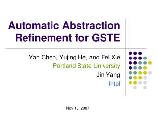
X 0 s 0 s 1 Generalized Symbolic Trajectory Evaluation (GSTE) • Based on gate-level simulation • Ternary simulation over {0,1,X} • Symbolic simulation layer • Fine control over abstraction • Fixed-points allow unbounded properties • Regular properties
Traditional Specification • Using assertion graphs • Shape and labels drive model checking • Affect efficiency and abstraction level Drive input A Assert correct output Drive input B
Verification Process High-level Specification An example specification For a simple GSTEproperty that isn’t too hard to verify I hope, but you never really know, Hopefully not Assertion Graph Manually Refine or Decompose GSTE Fails GSTE Succeeds Circuit
Verification Process Rules difficult to express, apply and justify High-level Specification An example specification For a simple GSTEproperty that isn’t too hard to verify I hope, but you never really know, Hopefully not Assertion Graph Manually Refine or Decompose GSTE Fails GSTE Succeeds Circuit
k b c k f f f Generalized Trajectory Logic • A clean specification notation based on temporal logic • Trace-based semantics • Symbolic set of words • What we check • GSTE simulation state • Upper-approximation • How we simulate
+ ( ( ) ) K N K S T S µ t 2 n r a c e s = ; Circuit Model • Kripke structure • Nodes
+ + + f ; b f k c k j j ( ( ) g ) g X ? X f f X f f X f X X X X X X S S S 0 1 t t 2 2 n n n n : ¾ ¾ s s : s s : : : : : : : : : : : Formulas of GTL
k b k b k b c c c k k k b b k k c c k k f X f f X X h h X X h h X h h X X X X 0 1 1 0 0 0 0 1 ^ _ t u t u \ [ g g g g g g = = Formulas of GTL
+ f k b c k ( b c ) j k k g f f f Y Y S t 2 2 g s ¾ e g g p s g ¾ g : Yesterday • Allows compositional simulation forward step simulate g
( b b ( j ) j j c ) ( ) c f f f h h h h l h l X X X X I Q Q Q Q 1 1 t n n n n e e g g u w : e u r u e g e n u g e a s s : e v : a u e u : u ! = ! ! = = = . . . . : : : : : : Symbolic Formulas
( ) ( ( ) ) ( ) f f h f f b d f f Y Z Z Z i i w e r e g n g s g e v e r y n ¹ g g ; ; : : : : Fixed-points • Mu-calculus style fixed-points capture iteration
( ) ( ( ( ) ) ) ( ) f f f h f f f b d f f f f P S Y Y Y Z Z Z Z Z Z Z i i _ _ ^ w e g r e : g : ¹ ¹ n g s g g e v e r y n ¹ g g = = ; ; : : : : : : Fixed-points • Mu-calculus style fixed-points capture iteration • E.g. ‘Previously f’ and ‘f Since g’
( ) Y Z E R O O N E t t _ ^ r e s e r e s e : = ( ) Y O N E Z E R O t ^ r e s e : = Vector Fixed-points • Nested mu-expressions are messy in practice • Fixed-points are unique • Can therefore use systems of recursive equations:
( ( ) ) ( ( ( ) ) ( j ( ) ) ) 9 f i f f Q Q T F _ n s n n u : : u : : u : = = = ! = : ( ) ( ( ) ) ( ( ) ) 8 f f f T F ^ u : u : u : = = = : Shorthand • Quantification • Calculated directly using BDD quantification • Symbolic node value
k ( ( k ) ( ( k k ) ) ) d l i d i d S A C A C i i i t t t ^ ^ 2 2 r e a w r w r n s o u s : m p e s ) ) GTL Properties when, for every trace t and in every symbolic valuation: e.g. Register correctness:
b c b c l A C A C i i v m p e s ) Model Checking Upper-approximation simulation Precise simulation, when C does not contain disjunction or Y
b c ( ) b c ( ( ( ) ) ) f f f f f f 6 f f f f f f f f Y Y Y Z Z Z Z ^ ^ ^ ^ ^ ^ n n ¹ g : g g g g ¹ g = = = = = = : : Reasoning with GTL • Simple rules for traced-based equivalence • Rules do not imply simulation equivalence • Property-preserving simulation transformations
( ) [ / ] f f f f f f Q Q ^ g u : u = = = Optimization Rules • Simplification, e.g. • Symbolic/explicit conversion
( ( ( j j ) ( ) ) ) ( ( j ) ( ) ) 9 1 0 _ _ n n n n n n n n n n n s s : s : : s : s : s : ! ! = ! = : Example 0 1 f s 1 f 1 1 f = =
A A B C B A C C A C A A B C C ) ) ) ) 1 1 2 2 2 1 2 1 A C [ = ] A A C C ) ) 2 1 1 2 Decomposition Rules • Transitivity connects simulations • Monotonicity connects branching simulations
( ( ) ) ( ) ( ) - - - f f f f h f f h Y Y Y Y _ ^ _ ^ _ g g g g g Abstraction Refinement • ‘Less abstract than’ relation • Only and lose information Information loss occurs earlier in simulation
a a a a a a a a a b b b b b b b b b ( ) b b b b b b Y Y Y Y Y ^ ^ ^ a a a a a a 1 1 1 1 1 1 1 1 • Affects which circuit segments are simulated independently
Conclusions • GTL is a temporal logic for GSTE • Textual form is easier to manage • Fine granularity induces algebraic nature • Logical rules express sound refinements • Simple rules exist for decomposition/refinement
( ) f f f f P S Y Y Z Z Z Z _ _ ^ g : : ¹ ¹ g = = : : • Previously f • f Since g
( ) Y Z E R O O N E t _ r e s e : = ( ) Y O N E Z E R O = • Fixed-points are unique • Can also use systems of equations, e.g.
I I µ [ [ \ \ m m Our Approach Assertion Graph: Simulation Steps: • Describe these atomic steps in a logical form • Hope to gain reasoning rules