Managing Cloud Resources: Distributed Rate Limiting
This workshop explores innovative methods for managing cloud resources through distributed rate limiting. Given the challenges of clients and resources distributed globally, the need for a central-like control over resource consumption is critical. We detail architectures such as token bucket limiters and global token buckets, emphasizing the importance of fairness in flow rates and responsiveness to application demands. The session covers engineering trade-offs and presents experiments highlighting the effectiveness of various rate limiting strategies in ensuring equitable resource usage across multiple TCP flows.

Managing Cloud Resources: Distributed Rate Limiting
E N D
Presentation Transcript
Managing Cloud Resources: Distributed Rate Limiting Alex C. Snoeren Kevin Webb, Bhanu Chandra Vattikonda, BarathRaghavan, KashiVishwanath, SriramRamabhadran,and Kenneth Yocum Building and Programming the Cloud Workshop 13 January 2010
Hosting with a single physical presence However, clients are across the Internet Centralized Internet services Mysore-Park Cloud Workshop – 13 January 2010
Cloud-based services • Resources and clients distributed across the world • Often incorporates resources from multiple providers Windows Live Mysore-Park Cloud Workshop – 13 January 2010
Resources in the Cloud • Distributed resource consumption • Clients consume resources at multiple sites • Metered billing is state-of-the-art • Service “punished” for popularity • Those unable to pay are disconnected • No control of resources used to serve increased demand • Overprovision and pray • Application designers typically cannot describe needs • Individual service bottlenecks varied but severe • IOps, network bandwidth, CPU, RAM, etc. • Need a way to balance resource demand Mysore-Park Cloud Workshop – 13 January 2010
Two lynchpins for success • Need a way to control and manage distributed resources as if they were centralized • All current models from OS scheduling and provisioning literature assume full knowledge and absolute control • (This talk focuses specifically on network bandwidth) • Must be able to efficiently support rapidly evolving application demand • Balance the resource needs to hardware realization automatically without application designer input • (Another talk if you’re interested) Mysore-Park Cloud Workshop – 13 January 2010
Ideal: Emulate a single limiter • Make distributed feel centralized • Packets should experience the same limiter behavior Limiters S D 0 ms S D 0 ms 0 ms S D Mysore-Park Cloud Workshop – 13 January 2010
Accuracy (how close to K Mbps is delivered, flow rate fairness) + Responsiveness (how quickly demand shifts are accommodated) Vs. Communication Efficiency (how much and often rate limiters must communicate) Engineering tradeoffs Mysore-Park Cloud Workshop – 13 January 2010
An initial architecture Limiter 1 Estimate interval timer Limiter 2 Packet arrival Gossip Limiter 3 Enforce limit Estimate local demand Gossip Gossip Limiter 4 Set allocation Global demand Mysore-Park Cloud Workshop – 13 January 2010
Token bucket limiters Packet Token bucket, fill rate K Mbps Mysore-Park Cloud Workshop – 13 January 2010
A global token bucket (GTB)? Demand info (bytes/sec) Limiter 1 Limiter 2 Mysore-Park Cloud Workshop – 13 January 2010
A baseline experiment Limiter 1 3 TCP flows Single token bucket D S 10 TCP flows D S Limiter 2 7 TCP flows S D Mysore-Park Cloud Workshop – 13 January 2010
GTB performance Global token bucket Single token bucket 10 TCP flows 7 TCP flows 3 TCP flows Problem: GTB requires near-instantaneous arrival info Mysore-Park Cloud Workshop – 13 January 2010
Take 2: Global Random Drop Limiters send, collect global rate info from others 5 Mbps (limit) 4 Mbps (global arrival rate) Case 1: Below global limit, forward packet Mysore-Park Cloud Workshop – 13 January 2010
Global Random Drop (GRD) 6 Mbps (global arrival rate) 5 Mbps (limit) Same at all limiters Case 2: Above global limit, drop with probability: Excess / Global arrival rate = 1/6 Mysore-Park Cloud Workshop – 13 January 2010
GRD baseline performance Global token bucket Single token bucket 10 TCPflows 7 TCP flows 3 TCP flows Delivers flow behavior similar to a central limiter Mysore-Park Cloud Workshop – 13 January 2010
GRD under dynamic arrivals Mysore-Park Cloud Workshop – 13 January 2010 (50-ms estimate interval)
Returning to our baseline Limiter 1 3 TCP flows D S Limiter 2 7 TCP flows D S Mysore-Park Cloud Workshop – 13 January 2010
Basic idea: flow counting Goal: Provide inter-flow fairness for TCP flows Local token-bucket enforcement “3 flows” “7 flows” Limiter 1 Limiter 2 Mysore-Park Cloud Workshop – 13 January 2010
Estimating TCP demand Localtoken rate (limit) = 10 Mbps 1 TCP flow S Flow A = 5 Mbps 1 TCP flow S Flow B = 5 Mbps Flow count = 2 flows Mysore-Park Cloud Workshop – 13 January 2010
FPS under dynamic arrivals Mysore-Park Cloud Workshop – 13 January 2010 (500-ms estimate interval)
Comparing FPS to GRD FPS(500-ms est. int.) GRD(50-ms est. int.) • Both are responsive and provide similar utilization • GRD requires accurate estimates of the global rate at all limiters. Mysore-Park Cloud Workshop – 13 January 2010
Estimating skewed demand Limiter 1 1 TCP flow S D 1 TCP flow S Limiter 2 3 TCP flows D S Mysore-Park Cloud Workshop – 13 January 2010
Estimating skewed demand Localtoken rate (limit) = 10 Mbps Flow A = 8 Mbps Bottleneckedelsewhere Flow B = 2 Mbps Flow count ≠ demand Key insight: Use a TCP flow’s rate to infer demand Mysore-Park Cloud Workshop – 13 January 2010
Estimating skewed demand Localtoken rate (limit) = 10 Mbps Flow A = 8 Mbps Bottleneckedelsewhere Flow B = 2 Mbps Local Limit Largest Flow’s Rate 10 8 = 1.25 flows = Mysore-Park Cloud Workshop – 13 January 2010
FPS example Global limit = 10 Mbps Limiter 1 Limiter 2 1.25flows 3flows Global limit x local flow count Total flow count Set local token rate = 10 Mbps x 1.25 1.25 + 3 = = 2.94 Mbps Mysore-Park Cloud Workshop – 13 January 2010
FPS bottleneck example Mysore-Park Cloud Workshop – 13 January 2010 Initially 3:7 split between 10 un-bottlenecked flows At 25s, 7-flow aggregate bottlenecked to 2 Mbps At 45s, un-bottlenecked flow arrives: 3:1 for 8 Mbps
Real world constraints • Resources spent tracking usage is pure overhead • Efficient implementation (<3% CPU, sample & hold) • Modest communication budget (<1% bandwidth) • Control channel is slow and lossy • Need to extend gossip protocols to tolerate loss • An interesting research problem on its own… • The nodes themselves may fail or partition • In an asynchronous system, you cannot tell the difference • Need to have a mechanism that deals gracefully with both Mysore-Park Cloud Workshop – 13 January 2010
Robust control communication Mysore-Park Cloud Workshop – 13 January 2010 7 Limiters enforcing 10 Mbps limit Demand fluctuates every 5 sec between 1-100 flows Varying loss on the control channel
Handling partitions Mysore-Park Cloud Workshop – 13 January 2010 Failsafe operation: each disconnected group k/n Ideally: Bank-o-mat problem (credit/debit scheme) Challege: group membership with asymmetric partitions
Following PlanetLab demand • Apache Web servers on 10 PlanetLab nodes • 5-Mbps aggregate limit • Shift load over time from 10 nodes to 4 5 Mbps Mysore-Park Cloud Workshop – 13 January 2010
Current limiting options Demands at 10 apache servers on Planetlab Wasted capacity Demand shifts to just 4 nodes Mysore-Park Cloud Workshop – 13 January 2010 31
Applying FPS on PlanetLab Mysore-Park Cloud Workshop – 13 January 2010 32
Hierarchical limiting Mysore-Park Cloud Workshop – 13 January 2010
A sample use case Mysore-Park Cloud Workshop – 13 January 2010 • T 0: A: 5 flows at L1 • T 55: A: 5 flows at L2 • T 110: B: 5 flows at L1 • T 165: B: 5 flows at L2
Worldwide flow join Mysore-Park Cloud Workshop – 13 January 2010 • 8 nodes split between UCSD and Polish Telecom • 5 Mbps aggregate limit • A new flow arrives at each limiter every 10 seconds
Worldwide demand shift Mysore-Park Cloud Workshop – 13 January 2010 • Same demand-shift experiment as before • At 50 sec, Polish Telecom demand disappears • Reappears at 90 sec.
Where to go from here • Need to “let go” of full control, make decisions with only a “cloudy” view of actual resource consumption • Distinguish between what you know and what you don’t know • Operate efficiently when you know you know. • Have failsafe options when you know you don’t. • Moreover, we cannot rely upon application/service designers to understand their resource demands • The system needs to dynamically adjust to shifts • We’ve started to manage the demand equation • We’re now focusing on the supply side: custom-tailored resource provisioning. Mysore-Park Cloud Workshop – 13 January 2010