Next Generation Sequencing

1. Next Generation Sequencing ImanHajirasouliha, 19 Oct 2012

2. Summery of today’s class • Next Generation Sequencing • Mapping short reads on to the reference genome • Human genome variation (SV) • Structural Variation discovery methods • Insertion and Deletion • Novel sequence insertions discovery • Mobile element insertions discovery • Simultaneous SV discovery among multiple genomes • Complexity, algorithms, 1000GP results Outline

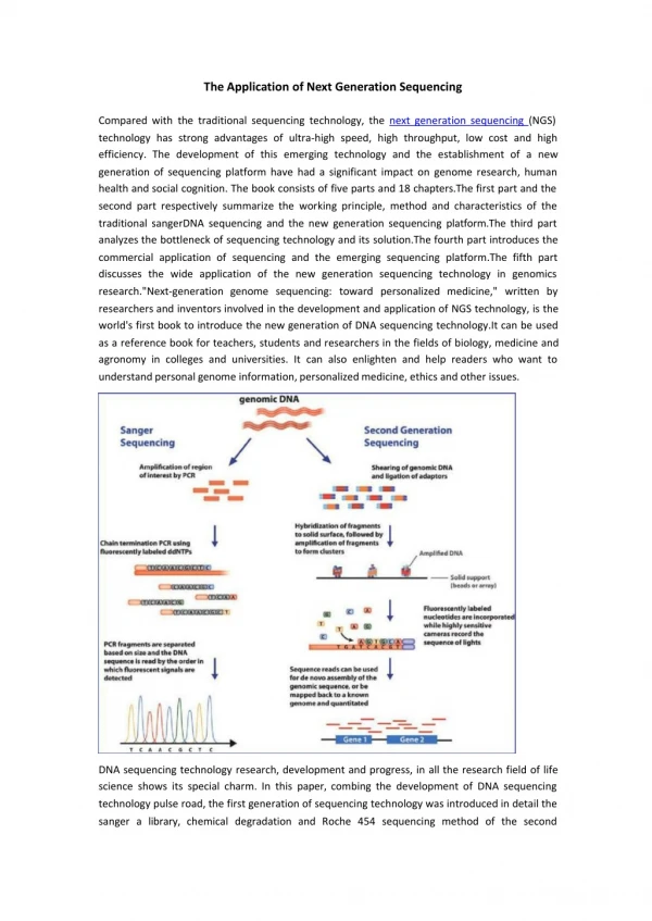
3. DNA sequencing How we obtain the sequence of nucleotides of a species …ACGTGACTGAGGACCGTG CGACTGAGACTGACTGGGT CTAGCTAGACTACGTTTTA TATATATATACGTCGTCGT ACTGATGACTAGATTACAG ACTGATTTAGATACCTGAC TGATTTTAAAAAAATATT…

4. Whole Genome Sequencing Test genome Random shearing and Size-selection Paired-end sequencing Read mapping Reference Genome (HGP) Maps to Forward strand Maps to Reverse strand

5. Whole Genome Sequencing Test genome Random shearing and Size-selection Paired-end sequencing Read mapping Reference Genome (HGP) Maps to Forward strand Maps to Reverse strand

6. NGS Technologies • 454 Life Sciences: the first, acquired by Roche • Pyrosequencing • Illumina (Solexa): current market leader • GAIIx, HiSeq2000, MiSeq, HiSeq2500 • Sequencing by synthesis • Applied Biosystems: • SOLiD: “color-space reads”

7. Features of NGS data • Short sequence reads • ~500 bp: 454 (Roche) • 35 – 150 bpSolexa(Illumina), SOLiD(AB) • Huge amount of sequence per run • Gigabases per run (600 Gbp for Illumina/HiSeq2000) • Huge number of reads per run • Up to billions • Bias against high and low GC content (most platforms) • GC% = (G + C) / (G + C + A + T) • Higher error (compared with Sanger) • Different error profiles

8. Next Gen: Raw Data • Machine Readouts are different • Read length, accuracy, and error profiles are variable. • All parameters change rapidly as machine hardware, chemistry, optics, and noise filtering improves

9. Current and future application areas Genome re-sequencing: somatic mutation detection, organismal SNP discovery, mutational profiling, structural variation discovery reference genome DEL SNP De novo genome sequencing • Sequencing is becoming an alternative to microarrays for: • DNA-protein interaction analysis (CHiP-Seq) • novel transcript discovery • quantification of gene expression • epigenetic analysis (methylation profiling)

10. Fundamental informatics challenges 1. Interpreting machine readouts – base calling, base error estimation 2. Data visualization 3. Data storage & management Gzip compressed raw data for one human genome > 100 GB

11. Informatics challenges (cont’d) 4. SNP, indel, and structural variation discovery 5. De novo Assembly

12. What can we use them for?

13. Mapping reads

14. Read Mapping (NGS) • When we have a reference genome & reads from DNA sequencing, which part of the genome does it come from? • Challenges: • Next-Gen sequencing: • Billions of short reads • Common: sequencing errors • More prevalent in NGS • Common: contamination • Typically ~2-3% of reads come from different sources; i.e. human resequencing contaminated with yeast, E. coli, etc. • Common: Repeats & Duplications

15. Read Mapping • Accuracy • Due to repeats, we need a confidence score in alignment • Sensitivity • Don’t lose information • Speed!!!!!!! • Think of the memory usage • Output • Keep all needed information, but don’t overflow your disks • All read mapping algorithms perform alignment at some point (read vs. reference)

16. Local vs. Global Alignment • The Global Alignment Problem tries to find the best alignment from start to end for two sequences • The Local Alignment Problem tries to find the subsequences of two sequences that give the best alignment • Solutions to both are extensions of Longest Common Subsequence

17. Local vs. Global Alignment (cont’d) • Global Alignment • Local Alignment—better alignment to find conserved segment --T—-CC-C-AGT—-TATGT-CAGGGGACACG—A-GCATGCAGA-GAC | || | || | | | ||| || | | | | |||| | AATTGCCGCC-GTCGT-T-TTCAG----CA-GTTATG—T-CAGAT--C tccCAGTTATGTCAGgggacacgagcatgcagagac |||||||||||| aattgccgccgtcgttttcagCAGTTATGTCAGatc

18. Percent Sequence Identity • The extent to which two nucleotide or amino acid sequences are invariant A C C T G A G – A G A C G T G – G C A G mismatch indel 70% identical

19. Global Alignment • Hamming distance: • Easiest; two sequences s1, s2, where |s1|=|s2| • HD(s1, s2) = #mismatches • Edit distance • Include indels in alignment • Levenstein’s edit distance algorithm, simple recursion with match score = +1, mismatch=indel=-1; O(mn) • Needleman-Wunsch: extension with scoring matrices and affine gap penalties; O(mn)

20. Edit Distance vs Hamming Distance Edit distance may compare i-th letter of v with j-th letter of w Hamming distance always compares i-th letter of v with i-th letter of w V = -ATATATAT V = ATATATAT W = TATATATA W = TATATATA - Hamming distance: Edit distance: d(v, w)=8d(v, w)=2 (one insertion and one deletion)

21. The Global Alignment Problem Find the best alignment between two strings under a given scoring schema Input : Strings v and w and a scoring schema Output : Alignment of maximum score ↑→ = -б = 1 if match = -µ if mismatch si-1,j-1 +1 if vi = wj si,j = max s i-1,j-1 -µ if vi ≠ wj s i-1,j - σ s i,j-1 - σ m : mismatch penalty σ : indel penalty {

22. Scoring matrices • Different scores for different character match & mismatches • Amino acid substitution matrices • PAM • BLOSUM • DNA substitution matrices

23. Scoring Matrices To generalize scoring, consider a (4+1) x(4+1) scoring matrixδ. In the case of an amino acid sequence alignment, the scoring matrix would be a (20+1)x(20+1) size. The addition of 1 is to include the score for comparison of a gap character “-”. This will simplify the algorithm as follows: si-1,j-1 + δ(vi, wj) si,j = max s i-1,j + δ(vi, -) s i,j-1 + δ(-, wj) {

24. Scoring Indels: Naive Approach • A fixed penalty σis given to every indel: • -σ for 1 indel, • -2σ for 2 consecutive indels • -3σ for 3 consecutive indels, etc. Can be too severe penalty for a series of 100 consecutive indels

25. This is more likely. This is less likely. Affine Gap Penalties • In nature, a series of k indels often come as a single event rather than a series of k single nucleotide events: ATA__GC ATATTGC ATAG_GC AT_GTGC Normal scoring would give the same score for both alignments

26. Accounting for Gaps • Gaps- contiguous sequence of spaces in one of the rows • Score for a gap of length x is: -(ρ +σx) where ρ >0 is the penalty for introducing a gap: gap opening penalty ρ will be large relative to σ: gap extension penalty because you do not want to add too much of a penalty for extending the gap.

27. Affine Gap Penalties • Gap penalties: • -ρ-σ when there is 1 indel • -ρ-2σ when there are 2 indels • -ρ-3σ when there are 3 indels, etc. • -ρ- x·σ (-gap opening - x gap extensions) • Somehow reduced penalties (as compared to naïve scoring) are given to runs of horizontal and vertical edges

28. Affine Gap Penalty Recurrences Continue Gap in w (deletion) si,j = s i-1,j - σ max s i-1,j –(ρ+σ) si,j = s i,j-1 - σ max s i,j-1 –(ρ+σ) si,j = si-1,j-1 + δ(vi, wj) max s i,j s i,j Start Gap in w (deletion): from middle Continue Gap in v (insertion) Start Gap in v (insertion):from middle Match or Mismatch End deletion: from top End insertion: from bottom

29. Ukkonnen’s Approximate String Matching Regular alignment Observation: If max allowed edit distance is small, you don’t go far away from the diagonal (global alignment only) AUUGACAGG - - AU - - - CAGGCC

30. Ukkonen’s alignment If maximum allowed number of indels is t, then you only need to calculate 2t-1 diagonals around the main diagonal.

31. there is only this change from the original recurrence of a Global Alignment - since there is only one “free ride” edge entering into every vertex The Local Alignment Recurrence • The largest value of si,j over the whole edit graph is the score of the best local alignment. • The recurrence: 0 si,j = max si-1,j-1 + δ(vi, wj) s i-1,j + δ(vi, -) s i,j-1 + δ(-, wj) { Smith-Waterman Algorithm

32. Smith-Waterman { 0 si,j = max si-1,j-1 + δ(vi, wj) s i-1,j + δ(vi, -) s i,j-1 + δ(-, wj) • Start from the maximum score s(i,j) on the alignment matrix • Move to m(i-1, j), m(i, j-1) or m(i-1, j-1) until s(i,j)=0 or i=j=0 • O(mn)

33. Faster Implementations • GPGPU: general purpose graphics processing units • Should avoid branch statements (if-then-else) • FPGA: field programmable gate arrays • SIMD instructions: single-instruction multiple data • SSE instruction set (Intel) • Also available on AMD processors • Same instruction is executed on multiple data concurrently

34. Alignment with SSE Genome seg(L-k+2) • Applicable to both global and local alignment • Using SSE instruction set we can compute each diagonal in parallel • Each diagonal will be in saved in a 128 bit SSE specific register • The diagonal C, can be computed from diagonal A and B in parallel • Number of SSE registers is limited, we cannot hold the matrix, but only the two last diagonals is needed anyway. x x x x x x x A x x x x A B C x x x R E A D (L-K) C A B x x x x C x x x x x x x x x x x x x x x x x x x

35. Mapping Reads Problem: We are given a read, R, and a reference sequence, S.Find the best or all occurrences of R in S. Example: R = AAACGAGTTA S = TTAATGCAAACGAGTTACCCAATATATATAAACCAGTTATT Considering no error: one occurrence. Considering up to 1 substitution error: two occurrences. Considering up to 10 substitution errors: many meaningless occurrences! Don’t forget to search in both forward and reverse strands!!!

36. Mapping Reads (continued) Variations: • Sequencing error • No error: R is a perfect subsequence of S. • Only substitution error: R is a subsequence of S up to a few substitutions. • Indel and substitution error: R is a subsequence of S up to a few short indels and substitutions. • Junctions (for instance in alternative splicing) • Fixed order/orientation R = R1R2…Rn and Rimap to different non-overlapping loci in S, but to the same strand and preserving the order. • Arbitrary order/orientation R = R1R2…Rn and Rimap to different non-overlapping loci in S.

37. Mapping algorithms • Two main “styles”: • Hash based seed-and-extend (hash table, suffix array, suffix tree) • Index the k-mers in the genome • Continuous seeds and gapped seeds • When searching a read, find the location of a k-mer in the read; then extend through alignment • Requires large memory; this can be reduced with cost to run time • More sensitive, but slow • Burrows-Wheeler Transform & Ferragina-Manzini Index based aligners • BWT is a data compression method used to compress the genome index • Perfect hits can be found very quickly, memory lookup costs increase for imperfect hits • Reduced sensitivity

38. “Long” read mappers • BLAST, MegaBLAST, BLAT, LASTZ can be used for Sanger, 454, Ion Torrent • Hash based • Extension step is done using Smith-Waterman algorithm • BLAST and MegaBLAST have additional scoring scheme to order hits and assign confidence values • 454/Ion Torrent only: PASH, Newbler

39. Short read mappers • Hash based • Illumina: mrFAST, mrsFAST, MAQ, MOSAIK, SOAP, SHRiMP, etc. • MOSAIK requires ~30GB memory • Others limit memory usage by dividing genome into chunks • mrFAST, SHRiMP have SSE-based implementation • MAQ: Hamming distance only • SOLiD: drFAST, BFAST, SHRiMP, mapreads • GPGPU implementations: Saruman, Mummer-GPU

40. Short read mappers • BWT-FM based • Illumina: BWA, Bowtie, SOAP2 • Human genome can be compressed into a 2.3 GB data structure through BWT • Extremely fast for perfect hits • Increased memory lookups for mismatch • Indels are found in postprocessing when paired-end reads are available • GPGPU implementations: SOAP3 (poor performance due to memory lookups)

41. Read mappers: PacBio • BLASR aligner; tuned for PacBio error model (indel dominated, ~15%) • Two versions: • Suffix array (hash) based • BWT-FM based

42. Hash Based Aligners

43. Seed and extend • Break the read into n segments of k-mers. • For perfect sensitivity under edit distance e • There is at least one l-mer where l = floor(L/(e+1)); L=read length • Forfixed l=k; n = e+1 and k ≤ L / n • Large k -> large memory • Small k -> more hash hits • Lets consider the read length is 36 bp, and k=12. • if we are looking for 2 edit distance (mismatch, indel) this would guaranty to find all of the hits

44. Human genome variation

45. Human genetic variation • Human genomes are different! • Single nucleotide polymorphisms (SNPs) • Few to ~50bp (small indels, microsatellites) • >50bp to several megabases (structural variants): • Deletions • Insertions • Novel sequence • Mobile elements (Alu, L1, SVA, etc.) • Segmental Duplications • Duplications of size ≥ 1 kbp and sequence similarity ≥ 90% • Inversions • Translocations • Complex (overlapping) events Introduction

46. Human genome structural variation • The pilot study of the 1000 genomes project reported: • 15 million SNPs • 1 million short indels • 20,000 structural variants (SVs) Introduction 46

47. Overview of SV discovery methods • Read pair analysis • Deletions, small novel insertions, inversions, transposons • breakpoint resolution dependents on the insert size • Read depth analysis • Deletions and duplications only • Relatively poor breakpoint resolution • Split read analysis • Small novel insertions/deletions, and mobile element insertions • 1bp breakpoint resolution • Local and de novo assembly • SV in unique segments • 1bp breakpoint resolution • Integrative models Introduction

48. Read Pair (RP) discovery methods • PEMer (Yale) developed mainly for Roche/454 data, uses BLAT to map reads to unique locations. Spanner (Boston College). and BreakDancer (Wash U) focus only on the “best mapping”. • Variation Hunter,Next Generation Variation Hunter (SFU/UW) consider multiple mappings.MoDil(UofT),GASV, GASV-pro (Brown) • GenomeSTRiP(Broad), MoGUL(UofT), CommonLAW(SFU): multiple- genome analysis (pooled) • Alkan et al. Genome structural variation discovery and genotyping, Nature Review Genetics (May 2011) Introduction

49. Paired-end mapping and SV detection Introduction Tuzun et al. 2005, Korbel et al. 2007, Alkan et al. 2011

50. RP methods and multiple mappings • Most methods consider unique or best mappings. • Ignoring repeats may mean that important biological phenomena are missed (Treangenand Salzberg, Nature Reviews Genetics, 2012). • Our methods (e.g. Variation Hunter and CommonLAW)consider multiple mappingsto handle the repeat regions. • Finding the correct mapping location of discordantpaired-end reads is challenging. Introduction