7. Excess Gibbs Energy Models

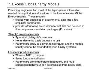
1. 7. Excess Gibbs Energy Models • Practicing engineers find most of the liquid-phase information needed for equilibrium calculations in the form of excess Gibbs Energy models. These models: • reduce vast quantities of experimental data into a few empirical parameters, • provide information an equation format that can be used in thermodynamic simulation packages (Provision) • “Simple” empirical models • Symmetric, Margule’s, vanLaar • No fundamental basis but easy to use • Parameters apply to a given temperature, and the models usually cannot be extended beyond binary systems. • Local composition models • Wilsons, NRTL, Uniquac • Some fundamental basis • Parameters are temperature dependent, and multi-component behaviour can be predicted from binary data. Lecture 21

2. Excess Gibbs Energy Models • Our objectives are to learn how to fit Excess Gibbs Energy models to experimental data, and to learn how to use these models to calculate activity coefficients. Lecture 21

3. Margule’s Equations • While the simplest Redlich/Kister-type expansion is the Symmetric Equation, a more accurate model is the Margule’s expression: • (12.9a) • Note that as x1 goes to zero, • and from L’hopital’s rule we know: • therefore, • and similarly Lecture 21

4. Margule’s Equations • If you have Margule’s parameters, the activity coefficients are easily derived from the excess Gibbs energy expression: • (12.9a) • to yield: • (12.10ab) • These empirical equations are widely used to describe binary solutions. A knowledge of A12 and A21 at the given T is all we require to calculate activity coefficients for a given solution composition. Lecture 21

5. van Laar Equations • Another two-parameter excess Gibbs energy model is developed from an expansion of (RTx1x2)/GE instead of GE/RTx1x2. The end results are: • (12.16) • for the excess Gibbs energy and: • (12.17a) • (12.17b) • for the activity coefficients. • Note that: as x10, ln1  A’12 • and as x2  0, ln2  A’21 Lecture 21

6. 8. Non-Ideal VLE to Moderate Pressure SVNA 14.1 • We now have the tools required to describe and calculate vapour-liquid equilibrium conditions for even the most non-ideal systems. • 1. Equilibrium Criteria: • In terms of chemical potential • In terms of mixture fugacity • 2. Fugacity of a component in a non-ideal gas mixture: • 3. Fugacity of a component in a non-ideal liquid mixture: Lecture 21

7. g, f Formulation of VLE Problems • To this point, Raoult’s Law was only description we had for VLE behaviour: • We have repeatedly observed that calculations based on Raoult’s Law do not predict actual phase behaviour due to over-simplifying assumptions. • Accurate treatment of non-ideal phase equilibrium requires the use of mixture fugacities. At equilibrium, the fugacity of each component is the same in all phases. Therefore, • or, • determines the VLE behaviour of non-ideal systems where Raoult’s Law fails. Lecture 21

8. Non-Ideal VLE to Moderate Pressures • A simpler expression for non-ideal VLE is created upon defining a lumped parameter, F. • The final expression becomes, • (i = 1,2,3,…,N) 14.1 • To perform VLE calculations we therefore require vapour pressure data (Pisat), vapour mixture and pure component fugacity correlations (i) and liquid phase activity coefficients (i). Lecture 21

9. Non-Ideal VLE to Moderate Pressures • Sources of Data: • 1. Vapour pressure: Antoine’s Equation (or similar correlations) • 14.3 • 2. Vapour Fugacity Coefficients: Viral EOS (or others) • 14.6 • 3. Liquid Activity Coefficients • Binary Systems - Margules,van Laar, Wilson, NRTL, Uniquac • Ternary (or higher) Systems - Wilson, NRTL, Uniquac Lecture 21