Volume Rendering using Graphics Hardware
Volume Rendering using Graphics Hardware. Travis Gorkin GPU Programming and Architecture, June 2009. Agenda. Volume Rendering Background Volumetric Data Optical Model Accumulation Equations Volume Rendering on the CPU Raymarching Algorithm Volume Rendering on Graphics Hardware

Volume Rendering using Graphics Hardware
E N D
Presentation Transcript
Volume Renderingusing Graphics Hardware Travis Gorkin GPU Programming and Architecture, June 2009
Agenda • Volume Rendering Background • Volumetric Data • Optical Model • Accumulation Equations • Volume Rendering on the CPU • Raymarching Algorithm • Volume Rendering on Graphics Hardware • Slice-Based Volume Rendering • Stream Model for Volume Raycasting • Volume Rendering in CUDA
Volume Rendering Definition • Generate 2D projection of 3D data set • Visualization of medical and scientific data • Rendering natural effects - fluids, smoke, fire • Direct Volume Rendering (DVR) • Done without extracting any surface geometry
Volumetric Data • 3D Data Set • Discretely sampled on regular grid in 3D space • 3D array of samples • Voxel – volume element • One or more constant data values • Scalars – density, temperature, opacity • Vectors – color, normal, gradient • Spatial coordinates determined by position in data structure • Trilinear interpolation • Leverage graphics hardware
Transfer Function • Maps voxel data values to optical properties • Glorified color maps • Emphasize or classify features of interest in the data • Piecewise linear functions, Look-up tables, 1D, 2D • GPU – simple shader functions, texture lookup tables
Volume Rendering Optical Model • Light interacts with volume ‘particles’ through: • Absorption • Emission • Scattering • Sample volume along viewing rays • Accumulate optical properties
Volume Ray Marching • Raycast – once per pixel • Sample – uniform intervals along ray • Interpolate – trilinear interpolate, apply transfer function • Accumulate – integrate optical properties
Ray Marching Accumulation Equations • Accumulation = Integral • Color Transmissivity = 1 - Opacity Total Color = Accumulation (Sampled Colors x Sampled Transmissivities)
Ray Marching Accumulation Equations • Discrete Versions • Accumulation = Sum • Color • Opacity Transmissivity = 1 - Opacity
CPU Based Volume Rendering • Raycast and raymarch for each pixel in scene • Camera (eye) location: • For Each Pixel • Look Direction: • Cast Ray Along: • Accumulate Color Along Line
CPU Based Volume Rendering • Sequential Process • Minutes or Hours per frame • Optimizations • Space Partitioning • Early Ray Termination
Volumetric Shadows • Light attenuated as passes through volume • ‘Deeper’ samples receive less illumination • Second raymarch from sample point to light source • Accumulate illumination from sample’s point of view • Same accumulation equations • Precomputed Light Transmissivity • Precalculate illumination for each voxel center • Trilinearly interpolate at render time • View independent, scene/light source dependent
GPU Based Volume Rendering • GPU Gems Volume 1: Chapter 39 • “Volume Rendering Techniques” • Milan Ikits, Joe Kniss, Aaron Lefohn, Charles Hansen • IEEE Visualization 2003 Tutorial • “Interactive Visualization of Volumetric Data on Consumer PC Hardware” • “Acceleration Techniques for GPU-Based Volume Rendering” • J. Krugger and R. Westermann, IEEE Visualization 2003
Slice-Based Volume Rendering (SBVR) • No volumetric primitive in graphics API • Proxy geometry - polygon primitives as slices through volume • Texture polygons with volumetric data • Draw slices in sorted order – back-to-front • Use fragment shader to perform compositing (blending)
Volumetric Data • Voxel data sent to GPU memory as • Stack of 2D textures • 3D texture • Leverage graphics pipeline • Instructions for setting up 3D texture in OpenGL • http://gpwiki.org/index.php/OpenGL_3D_Textures
Proxy Geometry • Slices through 3D voxel data • 3D voxel data = 3D texture on GPU • Assign texture coordinate to every slice vertex • CPU or vertex shader
Proxy Geometry • Object-Aligned Slices • Fast and simple • Three stacks of 2D textures – x, y, z principle directions • Texture stack swapped based on closest to viewpoint
Proxy Geometry • Issues with Object-Aligned Slices • 3x memory consumption • Data replicated along 3 principle directions • Change in viewpoint results in stack swap • Image popping artifacts • Lag while downloading new textures • Sampling distance changes with viewpoint • Intensity variations as camera moves
Proxy Geometry • View-Aligned Slices • Slower, but more memory efficient • Consistent sampling distance
Proxy Geometry • View-Aligned Slices Algorithm • Intersect slicing planes with bounding box • Sort resulting vertices in (counter)clockwise order • Construct polygon primitive from centroid as triangle fan
Proxy Geometry • Spherical Shells • Best replicates volume ray casting • Impractical – complex proxy geometry
Rendering Proxy Geometry • Compositing • Over operator – back-to-front order • Under operator – front-to-back order
Rendering Proxy Geometry • Compositing = Color and Alpha Accumulation Equations • Easily implemented using hardware alpha blending • Over • Source = 1 • Destination = 1 - Source Alpha • Under • Source = 1 - Destination Alpha • Destination = 1
Simple Volume Rendering Fragment Shader void main( uniform float3 emissiveColor, uniform sampler3D dataTex, float3 texCoord : TEXCOORD0, float4 color : COLOR) { float a = tex3D(texCoord, dataTex); // Read 3D data texture color = a * emissiveColor; // Multiply by opac }
Fragment Shader with Transfer Function void main( uniform sampler3D dataTex, uniform sampler1D tfTex, float3 texCoord : TEXCOORD0, float4 color : COLOR ) { float v = tex3d(texCoord, dataTex); // Read 3D data color = tex1d(v, tfTex); // transfer function }
Local Illumination • Blinn-Phong Shading Model Resulting = Ambient + Diffuse + Specular
Local Illumination • Blinn-Phong Shading Model • Requires surface normal vector • Whats the normal vector of a voxel? Resulting = Ambient + Diffuse + Specular
Local Illumination • Blinn-Phong Shading Model • Requires surface normal vector • Whats the normal vector of a voxel? Gradient • Central differences between neighboring voxels Resulting = Ambient + Diffuse + Specular
Local Illumination • Compute on-the-fly within fragment shader • Requires 6 texture fetches per calculation • Precalculate on host and store in voxel data • Requires 4x texture memory • Pack into 3D RGBA texture to send to GPU
Local Illumination • Improve perception of depth • Amplify surface structure
Volumetric Shadows on GPU • Light attenuated from light’s point of view • CPU – Precomputed Light Transfer • Secondary raymarch from sample to light source • GPU • Two-pass algorithm • Modify proxy geometry slicing • Render from both the eye and the light’s POV • Two different frame buffers
Two Pass Volume Rendering with Shadows • Slice axis set half-way between view and light directions • Allows each slice to be rendered from eye and light POV • Render order for light – front-to-back • Render order for eye – (a) front-to-back (b) back-to-front
First Pass • Render from eye • Fragment shader • Look up light color from light buffer bound as texture • Multiply material color * light color
Second pass • Render from light • Fragment shader • Only blend alpha values – light transmissivity
Scattering and Translucency • General scattering effects too complex for interactive rendering • Translucency result of scattering • Only need to consider incoming light from cone in direction of light source
Scattering and Translucency • Blurring operation • See GPU Gems Chap 39 for details
Performance and Limitations • Huge amount of fragment/pixel operations • Texture access • Lighting calculation • Blending • Large memory usage • Proxy geometry • 3D textures
Volume Raycasting on GPU • “Acceleration Techniques for GPU-Based Volume Rendering” • Krugger and Westermann, 2003 • Stream model taken from work in GPU Raytracing • Raymarching implemented in fragment program • Cast rays of sight through volume • Accumulate color and opacity • Terminate when opacity reaches threshold
Volume Raycasting on GPU • Multi-pass algorithm • Initial passes • Precompute ray directions and lengths • Additional passes • Perform raymarching in parallel for each pixel • Split up full raymarch to check for early termination
Step 1: Ray Direction Computation • Ray direction computed for each pixel • Stored in 2D texture for use in later steps • Pass 1: Front faces of volume bounding box • Pass 2: Back faces of volume bounding box • Vertex color components encode object-space principle directions
Step 1: Ray Direction Computation • Subtraction blend two textures • Store normalized direction – RGB components • Store length – Alpha component
Fragment Shader Raymarching • DIR[x][y] – ray direction texture • 2D RGBA values • P – per-vertex float3 positions, front of volume bounding box • Interpolated for fragment shader by graphics pipeline • s – constant step size • Float value • d – total raymarched distance, s x #steps • Float value
Fragment Shader Raymarching • DIR[x][y] – ray direction texture • 2D RGBA values • P – per-vertex float3 positions, front of volume bounding box • Interpolated for fragment shader by graphics pipeline • s – constant step size • Float value • d – total raymarched distance, s x #steps • Float value • Parametric Ray Equation • r – 3D texture coordinates used to sample voxel data
Fragment Shader Raymarching • Ray traversal procedure split into multiple passes • M steps along ray for each pass • Allows for early ray termination, optimization • Optical properties accumulated along M steps • Simple compositing/blending operations • Color and alpha(opacity) • Accumulation result for M steps blended into 2D result texture • Stores overall accumlated values between multiple passes • Intermediate Pass – checks for early termination • Compare opacity to threshold • Check for ray leaving bounding volume
Optimizations • Early Ray Termination • Compare accumulated opacity against threshold • Empty Space Skipping • Additional data structure encoding empty space in volume • Oct-tree • Encode measure of empty within 3D texture read from fragment shader • Raymarching fragment shader can modulate sampling distance based on empty space value
Performance and Limitations • More physically-based than slice-based volume rendering • Guarantees equal sampling distances • Does not incorporate volumetric shadows • Reduced number of fragment operations • Fragment programs made more complex • Optimizations work best for non-opaque data sets • Early ray termination and empty space skipping can be applied
Volume Rendering in CUDA • NVIDIA CUDA SDK Code Samples • Example: Basic Volume Rendering using 3D Textures • http://developer.download.nvidia.com/compute/cuda/sdk/website/samples.html#volumeRender
Volume Rendering in CUDA • 3D Slicer – www.slicer.org • Open source software for visualization and image analysis • Funded by NIH, medical imaging, MRI data • Currently integrating CUDA volume rendering into Slicer 3.2

![Real-Time Volume Graphics [03] GPU-Based Volume Rendering](https://cdn2.slideserve.com/4026797/real-time-volume-graphics-03-gpu-based-volume-rendering-dt.jpg)