Download
1 / 59
600 likes | 805 Vues
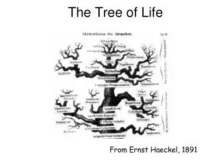
The Tree of Life. From Ernst Haeckel, 1891 . Phylogenetic Analysis. Classical approach considers morphological features number of legs, lengths of legs, etc. Modern approach considers molecular features gene sequences protein sequences

E N D
The Tree of Life From Ernst Haeckel, 1891
Phylogenetic Analysis • Classical approach considers morphological features • number of legs, lengths of legs, etc. • Modern approach considers molecular features • gene sequences • protein sequences • Use of molecular data provides objective criteria for constructing phylogenetic trees
Phylogenetic Analysis Phylogenetic analysis is based on homologous sequences in different species (e.g., globins) Sequences can be homologous for different reasons: orthologs -- sequences diverged after a speciation event paralogs-- sequences diverged after a duplication event xenologs -- sequences diverged after horizontal transfer (e.g., by virus)
Tree Terminology • A tree is a collection of nodes and edges with no cycles (i.e. there is no path from a node to itself) • Tree topology refers to the “shape” of the tree tree not a tree topologically equivalent
Tree Terminology • A tree is a collection of nodes and edges with no cycles (i.e. there is no path from a node to itself) • Classification of nodes (in the context of phylogenetic trees) • root – (a single distinguished node) represents the common ancestor • internal nodes – represent intermediate ancestors in the course of evolution • leaves – (the non-branching nodes) represent the species for which the tree is built tree not a tree
Tree Terminology • Rooted Trees • internal nodes have 3 edges (1 for parent, 2 for children) • a special node (the root) has 2 edges • the leaves (the given taxa) have one edge • Unrooted trees – same as above but do not have root node
Tree Terminology • Classification of nodes (in the context of phylogenetic trees) • root – (a single distinguished node) represents the common ancestor • internal nodes – represent ancestors in the course of evolution • leaves – (the non-branching nodes) represent the species for which the tree is built • When the root node is not specified the tree is unrooted
Counting Trees B A C A C B D D • How many trees are there that have n leaf nodes (or taxa)? Three Leaf Nodes B A C Only one unrooted tree is possible Four Leaf Nodes C B A D Three different unrooted trees are possible
Counting Trees • How many trees are there that have n leaf nodes (or taxa)? • NR = Number of possible rooted trees • = • NU = Number of possible unrooted trees • =
Tree Explosion The number of possible rooted trees for 15 different taxa is 213,458,046,767,875 Assuming a computer can create a tree in 10-9 seconds, it would take 2.47 days of computation time to create them. For 20 taxa, there are 8,200,794,532,637,891,559,337 possible trees and the same computer would take 259,867 years to generate this many trees!
Algorithms • Distance-based • UPGMA – Unweighted Pair-Group Mathod with Arithmetic Means • Fitch-Margoliash (FM) • Neighbor-Joining • Character-based • Maximum parsimony algorithm
Distance Data • Distance-based algorithms expect as input a matrix of distances (dij) between each pair of sequences • Distance data can be generated from the available sequences and models of base substitution • Jukes-Cantor model • p – fraction of mismatches • Kimura model • P – fraction of transitions • Q – fraction transversions
UPGMA Algorithm • Main idea: Group the taxa into clusters and repeatedly merge the closest two clusters until one cluster remains • Algorithm • Add a leaf to the tree for each taxon • Initially make each taxon be its own cluster • Find the closest clusters and connect with node in the tree (place new node at equal distance from the clusters) • Repeat previous step until all clusters are connected x4 x2 x3 x5 x1 root x2 x1 x3 x5 x4
UPGMA Clustering • The algorithm needs to compute distance between clusters • The distance between clusters Ci and Cj is defined to be the average distance between all pairs of taxa in Ci and Cj
UPGMA Clustering • The algorithm needs to compute distance between clusters • The distance between clusters Ci and Cj is defined to be the average distance between all pairs of taxa in Ci and Cj • Shortcut when combining Ci and Cj to form new cluster Ck
UPGMA Assume the following distance matrix Closest Pair is {x3, x5} so cluster them, C1 = {x3,C5} Add new node for x3, x5 at height d(x3,x5) / 2 = 1 Compute the distance from C1 to the rest d(C1,x1) = 1/2 (d(x3,x1) + d(x5,x1) ) = 6 d(C1,x2) = 1/2 (d(x3,x2) + d(x5,x2) ) = 16 d(C1,x4) = 1/2 (d(x3,x4) + d(x5,x4) ) = 16 1 1 x3 x5
UPGMA The updated distance matrix – C1 replaced x3, x5 Closest Pair is {x1, C1} so cluster them, C2 = {x1,C1} Add new node for x1, C1 at height d(x1,C1) / 2 = 3 Compute the distances from C2 to the d(C2,x2) = 1/3 (d(x1,x2) + d(x3,x2) +d(x5,x2) ) = 16 d(C2,x4) = 1/3 (d(x1,x4) + d(x3,x4) +d(x5,x4) ) = 16 2 3 1 1 x1 x3 x5
UPGMA The updated distance matrix – C2 replaced x1, C1 Closest Pair is {x2, x4} so cluster them, C3 = {x2,x4} Add new node for x2, x4 at height d(x2,x4) / 2 = 4 Compute the distances from C3 to the rest d(C3,C2) = 1/6 (d(x2,x1) + d(x2,x3) +d(x2,x5) + d(x4,x1) + d(x4,x3) +d(x4,x5)) = 16 2 4 4 3 1 1 x2 x1 x3 x5 x4
UPGMA The updated distance matrix – C3 replaced x2, x4 root Closest Pair is {C2, C3} so cluster them, C4 = {C2,C3} Add new node for C2, C3 at height d(C2,C4) / 2 = 8 5 4 Done! Double-check if original distances between taxa are preserved (not guaranteed) 2 4 4 3 1 1 x2 x1 x3 x5 x4
UPGMA Summary • Distance-based algorithm that produces rooted trees • Assumes that all species evolve at the same rate • (molecular clock hypothesis) • Implication of molecular clock hypothesis is that • distance from root to any taxon is the same • Final tree may not preserve original • distances between the taxa root 5 4 2 4 4 3 1 1 x2 x1 x3 x5 x4
FM Algorithm • Similar to UPGMA but removes molecular clock assumption • (i.e. distance from an internal node to leaves differs) • Produces unrooted trees • Algorithm (similar to UPGMA) • Add a leaf to the tree for each taxon • Initially make each taxon be its own cluster • Find the closest clusters and connect with node in the tree • (place new node at equal distance from the clusters • at distance given by 3-point formula) • Repeat previous step until all clusters are connected
FM and 3-point formula • Given three taxa i, j, k with distances d(i, j), d(i, k), d(j, k) • where should the interior node m be placed to connect the • taxa and preserve the distances? k j m i
FM and 3-point formula • Given three taxa i, j, k with distances d(i, j), d(i, k), d(j, k) • where should the interior node m be placed to connect the • taxa and preserve the distances? k j m i
FM Algorithm • Algorithm (similar to UPGMA) • Add a leaf to the tree for each taxon • Initially make each taxon be its own cluster • Find the closest clusters and connect with node in the tree (place new at distance given by 3-point formula, where the points are clusters of tax and we use the distance between clusters) • Repeat previous step until all clusters are connected x4 x2 x3 x5 x1 x1 x5 x4 x3 x2
Apply the FM algorithm to the following distance matrix: A and B are closest; temporarily group C-D-E and compute d(A, B), d(A, C-D-E), d(B, C-D-E) to apply 3-point formula d(A,C-D-E) = 1/3(1.01+.75+1.03) = .93 d(B,C-D-E) = 1/3(1.00+.69+.90) = .863 d(A, B) = .31 A only used to help us group A, B .1885 By 3-point formula: .7415 C-D-E X d(C-D-E,X) = 1/2(d(C-D-E,A) + d(C-D-E,B) – d(A,B)) d(B, X) = 1/2(d(B,A) + d(B,C-D-E) – d(A,C-D-E)) d(A, X) = 1/2(d(A,B) + d(A,C-D-E) – d(B,C-D-E)) .1215 B
A and B are combined in a cluster for the rest of the algorithm, so need to recompute the distances from A-B to other clusters: d(A-B,C) = 1/2(1.01 + 1.00) = 1.005 d(A-B,D) = 1/2(.75 +.69) = .72 d(A-B, E) = 1/2(1.03 + .90) = .965 The updated table is: A .1885 The partial tree so far is: .1215 B
Based on the updated table D and E are closest; temporarily group A-B-C and compute d(D, E), d(D, A-B-C), d(E, A-B-C) to apply 3-point formula d(D,A-B-C) = 1/3(.75+.69+.61) = .683 d(E,A-B-C) = 1/3(1.03+.90+.42) = .783 d(D, E) = .37 only used to help us group D, E D .135 By 3-point formula: .548 A-B-C Y d(A-B-C,Y) = 1/2(d(A-B-C, D) + d(A-B-C,E) – d(D,E)) d(D, Y) = 1/2(d(D,E) + d(D,A-B-C) – d(E,A-B-C)) d(E, Y) = 1/2(d(E,D) + d(E,A-B-C) – d(D,A-B-C)) .235 E
D and E are combined in a cluster for the rest of the algorithm, so need to recompute the distances from D-E to other clusters: D A .1885 .135 d(A-B,D-E) = 1/4 (.75+1.03+.69+90) = .8425 d(A-B,C) = 1/2(1.01 + 1.00) = 1.005 d(C,D-E) = 1/2 (.61+.42) = .515 .235 .1215 E B The updated table is now: The partial tree so far is:
Based on the updated table There are only three clusters, so just apply the 3-point formula d(A-B,Z) = 1/2(d(A-B, D-E) + d(A-B,C) – d(D-E,C)) d(D-E,Z) = 1/2(d(D-E,A-B) + d(D-E,-C) – d(A-B,C)) d(C, Y) = 1/2(d(C,A-B) + d(C,D-E) – d(A-B,D-E)) C .33875 .66625 A-B Z .17625 D-E
Now we need to expand the clusters A-B, D-E C .33875 a Z b Z .135 D .235 E We also need to compute the values for a and b: C d(A-B, Z) = 1/2 (d(A,Z) + d(B, Z)) = 1/2 (.1885+a + .1215+a) = .66625 a = .51125 .33875 A .66625 d(D-E, Z) = 1/2 (d(D,Z) + d(E, Z)) = 1/2 (.235+b + .135+b) = .17265 b = -.00875 A-B .1885 .17625 The negative value for b is a cause for concern about the quality of the data. If we are confident of our data and since .00875 is close to 0, b would be set to 0. D-E .1215 B
FM Summary • Distance-based algorithm that produces unrooted trees • Removes the assumption of molecular clock, but does not give information about the root (common ancestor) • To detect the root could introduce an extra taxon (outgroup) that is more distantly related to the given taxa
NJ Algorithm • Similar to FM (also removes molecular clock assumption) • but more sophisticated in how it selects clusters to join • Produces unrooted trees • Algorithm (similar to FM) • Add a leaf to the tree for each taxon • Initially make each taxon be its own cluster • Find the closest clusters (using more sophisticated criterion) • (place new node at distance given by a variant of 3-point formula) • Repeat previous step until all clusters are connected
NJ “closeness” Criterion • Suppose that you are given n taxa x1, x2, x3, …, xn, and suppose that you have some tree that fits the distance data x5 x4 x3 x1 z y x6 x2 observation: d(x1,x2) + d(xi,xj) < d(x1,xi) + d(x2,xj) (right side includes yz twice, left does not)
NJ “closeness” Criterion d(x1,x2) + d(xi,xj) < d(x1,xi) + d(x2,xj) • From previous slide d(x1,x2) + d(x3,x4) < d(x1,x3) + d(x2,x4) For a fixed i, say i = 3: d(x1,x2) + d(x3,x5) < d(x1,x3) + d(x2,x5) d(x1,x2) + d(x3,x6) < d(x1,x3) + d(x2,x6) … … … d(x1,x2) + d(x3,xn) < d(x1,x3) + d(x2,xn) ------------------------------------------------- Add d(x3,x1),d(x3,x2) , d(x3,x3), d(x2,x1), d(x2,x2) to both sides
NJ “closeness” Criterion • From previous slide, if x1 and x2 are neighbors • Let • Then in general, if xk and xl are neighbors • NJ uses this observation to determine “closeness” and computes the smallest value M(k, l) to determine a cluster • Unlike UPGMA and FM, NJ has a more global view of “closeness” when selecting neighbors
NJ new node Placement • If x1 and x2 are neighbors; where should new node y be by 3-point formula x4 x5 x3 … … … x1 -------------------------------------------------------------- y x2 add on right side d(x1,x1 ) + d(x1,x2) - d(x2,x1 ) - d(x2,x2 )
NJ mini summary • For each pair of nodes xk and xl compute the quantity • Actually, could compute • When xk and xl are replaced by new node y, place y at • From now on Si will always be divided implicitly by (n-2)
NJ Algorithm • From the distance matrix compute the criterion matrix • Find the smallest value in M(i, j) – cluster the corresponding pair • Connect taxa xi and xj with a new node y placed at distance • Remove xi and xj and replace with y; update the distance matrix using the 3-point formula • Repeat from beginning
Apply the NJ algorithm to the given distance matrix: First compute Si=sum-of-row / (n-2) S1= 11.75 S2=10.25 S3=12.75 S4=14.25 S5=11.25 S6= 12.25 Compute M(1,2) = d(1,2) – S1 – S2 = 8 – 22= -14 M(1,3) = d(1,3) – S1 – S3 = 3 – 24.5= -21.5 M(1,4) = d(1,4) – S1 – S4 = 14 – 26 = -12 M(1,5) = d(1,5) – S1 – S5 = 10 – 23 = -13 M(1,4) = d(1,4) – S1 – S4 = 12 – 24 = -12 and so on … Find min value, i.e. the pair to cluster
From previous slide we need to cluster x1 and x3 Add a new taxon x7 and place it at distance Recompute distances from x7 to all others using the 3-point formula x3 x1 2 1 x7 d(7,2) = ½(d(1,2) + d(3,2) – d(1,3)) = 7 d(7,4) = ½(d(1,4) + d(3,4) – d(1,3)) = 13 d(7,5) = ½(d(1,5) + d(3,5) – d(1,3)) = 9 d(7,6) = ½(d(1,6) + d(3,6) – d(1,3)) = 11
Apply the NJ algorithm to the new distance matrix: First compute Si=sum-of-row / (n-2) S2= S4= S5= S6= S7= Compute M(2,4) = d(2,4) – S2 – S4 = M(2,5) = d(2,5) – S2 – S5 = M(2,6) = d(2,6) – S2 – S6 = M(2,7) = d(2,7) – S2 – S7 = and so on … Find min value, i.e. the pair to cluster
From previous slide we need to cluster ? and ?? Add a new taxon x8 and place it at distance Recompute distances from x8 to all others using the 3-point formula x?? x? ? ? x8
NJ Summary • Distance-based algorithm that produces unrooted trees • Removes the assumption of molecular clock, but does not give information about the root (common ancestor) • Typically performs better than UPGMA and FM – uses a more global criterion to select pairs to cluster • To detect the root could introduce an extra taxon (outgroup) that is more distantly related to the given taxa
Maximum Parsimony (MP) Algorithm