Download
1 / 70
730 likes | 1.08k Vues
Current Issues in Estimating the Cost of Capital for Electric Utilities. Prepared for EEI Electric Rates Advanced Course Madison, Wisconsin. by The Brattle Group 44 Brattle Street Cambridge, MA 02138 August 5, 2008. Overview of Presentation. Cost of Capital defined What is Risk?

E N D
Current Issues in Estimating the Cost of Capital for Electric Utilities Prepared for EEI Electric Rates Advanced Course Madison, Wisconsin by The Brattle Group 44 Brattle Street Cambridge, MA 02138 August 5, 2008
Overview of Presentation • Cost of Capital defined • What is Risk? • A brief review of utility Cost of Capital analysis • Standard estimation methods • Pitfalls of the standard models • Challenging issues for estimating the Cost of Capital for regulated electric utility companies. • Adjusting for financial risk • Increased regulated risks due to spill-over from deregulated generation market and now the move toward re-regulation in some states, e.g., VA, MT • Some recent issues with cost of equity methodologies • Off balance sheet obligations
Cost of Capital • Definition: Cost of Capital is the expected rate of return in capital markets for alternative investments of corresponding risk. • Supreme Court rulings provide guidelines for cost of capital analysis. A fair Cost of Capital must meet three requirements: • Commensurate with returns on enterprises with corresponding risks; • Sufficient to maintain the financial integrity of the regulated company; and • Adequate to allow the company to attract capital on reasonable terms.
Supreme Court Rulings on Cost of Capital • “The return should be reasonably sufficient to assure confidence in the financial soundness of the utility and should be adequate, under efficient and economical management, to maintain and support its credit and enable it to raise the money necessary for the proper discharge of its public duties.” (Bluefield Water Works & Improvement Company vs. Public Service Commission of West Virginia, 1923) • “[T]he return to the equity owner should be commensurate with returns on investments in other enterprises having corresponding risks. That return, moreover, should be sufficient to assure confidence in the financial integrity of the enterprise, so as to maintain its credit and to attract capital.” (Federal Power Commission vs. Hope Natural Gas Company, 1944)
Supreme Court Rulings (continued) • A regulated company “is entitled to such rates as will permit it to earn a return on the value of the property which it employs . . . equal to that generally being made . . . on investments in other business undertakings which are attended by corresponding risks and uncertainties.” (Bluefield Water Works & Improvement Company vs. Public Service Commission of West Virginia, 1923)
Components of Cost of Capital • Standard utility rate of return analysis requires the following components: • Rate Base: In the U.S., most utilities are regulated on the basis of an original cost rate base; thus, regulators use the book value capital structure of the regulated entity or its parent company; • Cost of Debt and Preferred Equity: standard practice in utility regulation is to use the embedded cost of debt and preferred; and • Cost of Equity: investors’ expected return on equity, now usually estimated from current market information. • Estimating the cost of equity is often one of the most controversial issues in a rate proceeding.
What is risk? • Many ways to look at risk: • “Things that can go wrong.” • “Undiversifiable” (“market,” “systematic”) vs. “diversifiable” (“unique,” “unsystematic”). • “Business” vs. “financial.” • “Symmetric” vs. “asymmetric.” • Answering the question with regard to estimating the Cost of Capital requires careful attention to the different type or types of risk.
Diversifiable vs. Undiversifiable Risk • Investors can reduce risk by holding portfolios instead of individual stocks. • The part that can be eliminated by holding a stock in a portfolio is the “diversifiable” risk. • But some risk remains, because stock returns depend in part on broad risk factors, such as the state of the economy. • The part that remains is the “undiversifiable” risk. • Finance theory holds that a stock’s required rate of return depends on the stock’s relative exposure to one or more undiversifiable risk factors that potentially affect all stocks.
Total vs. Undiversifiable Risk as the Number of Stocks in Portfolio Increases 40% 35% Total Risk 30% 25% Relative Risk 20% 15% Diversifiable Undiversifiable 10% Risk Risk 5% 0% 0 5 10 15 20 25 30 35 Number of Stocks in Portfolio Total vs. Undiversifiable Risk
Business vs. Financial Risk • In modern finance theory, a stock’s “business” risk is the risk shareholders would bear if the company in question used no debt. • The stock’s “financial” risk is the extra risk shareholders bear if the company uses debt. • The level of financial risk increases, and at an increasing rate, as companies add debt.
Illustrative Effect of Financial Risk on the Cost of Equity 20% Level due to Cost of Equity Business Risk 15% Effect of Financial Risk 10% Cost of Capital 5% Overall After-Tax Cost of Capital 0% 0 0.2 0.4 0.6 0.8 1 (Market) Debt/Value Ratio Illustration of Effect of Financial Risk
Symmetric vs. Asymmetric Risk • Rate regulation prevents extraordinarily good outcomes. • Therefore, it should also prevent extraordinarily bad outcomes. • Sometimes, however, extraordinarily bad outcomes happen to rate-regulated companies anyway. • Power plant cost overruns of the 1970s-80s. • Natural gas pipeline “take or pay” disputes in the 1980s. • California energy crisis of 2000-2001. • PoLR responsibility with rate caps 2005-2006 • Such risks may or may not affect the cost of capital, but they definitely affect the company’s opportunity to earn it.
No Bad Event, RoR = CoC on average. Start of Year Average outcome less than CoC Bad Event, RoR much less than CoC Example of Asymmetric Risk Fair expected rate of return (RoR) on utility rate base is the cost of capital (CoC). That is the breakeven RoR that the utility should expect to earn on average. But if there is a chance of a very bad event that is not offset by an equal chance for a very good event, the utility will expect less than the CoC on average.
Asymmetric Risk (continued) • Asymmetric risk in rate regulation is potentially a “big topic”. For example: • An asymmetric risk may or may not affect the cost of capital, depending on whether the “bad outcome” loss gets worse in bad economic times. • Nonetheless, an asymmetric risk must be remedied, or the utility is denied a fair opportunity to earn its cost of capital. • Several types of remedies exist; however, this presentation focuses on estimating the Cost of Capital, so asymmetric risk is discussed further.
Summary of Impact of Risk Types • Risk TypeRisk Effect • Undiversifiable: Affects cost of capital (CoC). • Diversifiable: Does not affect CoC. • Business: Affects overall cost of capital and cost of equity. • Financial: Affects cost of equity. • Asymmetric: 1. May or may not affect CoC. • 2. Requires a remedy if company is to • have a fair opportunity to earn CoC. • Symmetric: No effect not already considered above.
Cost of Equity Methodologies • Discounted Cash Flow (DCF) • Risk Positioning Models: • Risk Premium Method • Capital Asset Pricing Model (CAPM) (a “single-[risk]-factor” model) • Multi-[risk]-Factor models (e.g., Fama-French) • Arbitrage Pricing Theory (APT) • Comparable Earnings Model
DCF Method — Components • The simplest version of the model is Cost of Equity = • dividend yield (current income) + growth rate (i.e., capital gains) • Dividend yields can be easily calculated from market prices and the current dividend.
Discounted Cash Flow (DCF) • The value (current price) of a stock is often thought of as the present value of its expected dividend stream, discounted at the cost of equity. • When this is true (and it is not always), the cost of equity can be inferred from the stock price and expected dividends. • Often characterized as a “forward looking” estimate of the cost of equity because it relies upon investors’ expectations of future dividends, primarily by estimating one or more dividend growth rates. • Future growth of dividends cannot be observed directly, but must be inferred. • At some point in the dividend forecast, and often immediately, most DCF applications assume dividends will grow forever afterwards at a steady rate.
é ù 1 2 æ ö æ ö + + D D 1 g 1 g ç ÷ ç ÷ ê ú = + + = + + 1 2 P ... D ... ç ÷ ç ÷ ( ) ( ) 0 0 + + 1 2 + + 1 r 1 r ê ú 1 r 1 r è ø è ø ë û E E E E ( ) + D 1 g = 0 ( ) - r g E ( ) + 1 g D 0 = + r g E P 0 Discounted Cash Flow (DCF) Method • Simple model derived as follows: • Assumes current price of stock is the present value of its dividend stream, discounted at cost of equity • Observe current stock price and dividend (P0, D0) • Must estimate g (e.g. from data sources such as Value Line or Bloomberg)
DCF Method — Dividend Growth Rates • But expected future dividends must be estimated somehow. Some methods are: • To use analysts’ earnings growth rate forecasts as a proxy (Thomson’s Financial, Bloomberg or Value Line) • To use historical growth rates of dividends, earnings or other variables (not recommended) • Sustainable growth = RoE × Retention Ratio • Plus possibly: (% Growth in # of Shares) × (Market-to-Book ratio – 1) • FERC prefers a weighted average of the short-term analysts’ forecasts (2/3) and long-run GDP growth rate forecasts (1/3) for natural gas pipelines, but uses analyst forecasts and sustainable growth rate estimates for electric utilities.
DCF Model Issues • Assumes constant perpetual growth, which is problematic both theoretically and empirically: • Generally, there are no data on growth rates for periods farther than 5 years into the future; • However, the growth rate is the most important and often the most subjective parameter in the model. • Assumes no or very small option value reflected in stock prices • Net present value formulas do not apply to companies with strong growth options or in financial distress. • Hence, DCF cost of equity does not work for these companies.
D D D P 1 2 5 5 = + + + + P . . . + + + + 0 1 2 5 5 ( 1 r ) ( 1 r ) ( 1 r ) ( 1 r ) E E E E where D 6 = P - 5 ( r g ) E LR Two-Stage DCF Model Can also forecast near-term dividends to grow at different rates, then add a terminal value (“P5” below); this is called a “two-stage” or “multi-stage” DCF model: gLR is the perpetual growth rate. There are many variations on the multistage DCF model; often use perpetual long-run growth rate assumption to get terminal value, as is done here, but could also substitute some other estimate of the final price, if available.
Risk Positioning Approach • The common feature to this approach is to add a risk premium to a benchmark interest rate: • Simple risk premium model • Capital Asset Pricing Model (CAPM) • Multi-Factor Models (e.g., Fama-French) • Arbitrage Pricing Theory (APT) • The risk premium is usually based on historical information. • Multi-factor Models and APT attempt to improve upon the simple risk premium model by relying upon additional risk factors.
Simple Risk Premium Model • Cost of Equity = interest rate + risk premium • Interest rate is usually the yield on a Government bond or a corporate bond index. • Risk premium is estimated in a number of ways, in practice, including: • the historical average excess return* on a utility portfolio • the expected cost of equity estimated from DCF models on a broad stock index, minus the interest rate • the risk premium used last time by a particular commission • * “Excess return” is the actual return on a stock minus the risk-free interest rate, in some particular period; it may be positive or negative.
Cost of Capital E(rM) MRP CAPM Line rF Beta 1.0 Capital Asset Pricing Model (CAPM) • Expected return on equity (i.e., the cost of equity capital) is equal to the excess of the expected return on the market over the risk-free rate (known as the “market risk premium”, or “MRP”) times the stock’s beta (a measure of the relative risk of the stock), plus the risk-free rate. CAPM formula: E(rE) = rF +βE[E(rM) – rF] = rF +βE[MRP]
A CAPM Issue: Empirical Tests • The CAPM is a Nobel-Prize winning theory, and it has been the subject of numerous empirical tests; unfortunately, the results are mixed. • Stock returns do appear to be positively related to beta, as the CAPM predicts. • However, they are not as strongly correlated with beta as the CAPM predicts. • The actual intercept of a plot of beta versus the cost of capital lies above the risk-free rate, which means that low-beta stocks tend to have higher costs of capital and high-beta stocks lower costs of capital than predicted by the CAPM. • The graph on the next page illustrates this finding, which leads to another cost of capital estimation method: the Empirical CAPM.
Theoretical Capital Asset Pricing Model Vs. Relationship Found in Empirical Studies CAPM Security Market Line Cost of Capital Empirical Relation Average Cost of Capital CAPM Lower Than Empirical Line for Low Beta Stocks Market Risk Premium Risk-Free Interest Rate Beta Below 1.0 1.0 Beta Empirical CAPM
CAPM — Market-Wide Components • Risk-free rate: In rate cases, usually measured by the yield on either U.S. Government Treasury Bills or long-term Treasury Bonds. • Market Risk Premium: • In the past, usually estimated as the arithmetic average of the total return on the market portfolio minus the return on the risk-free asset for as a long a period as permitted by data availability. • Currently very controversial. Some argue that magnitude of the historical average MRP is too large. • Some argue that MRP is not constant through time, i.e., that the MRP: • Varies with interest rates. • Varies with expected variability of the market. • Varies with some other factor. • Should be consistent with the risk-free interest rate used.
CAPM Beta • Beta measures the sensitivity of an individual stock to fluctuations in the market: • High-beta stocks exaggerate the market’s fluctuations. • Low-beta stocks respond less-than-proportionately to market fluctuations. • According to CAPM (and all modern models of the cost of capital), only non-diversifiable risks (measured by beta, or “betas,” in multi-factor models) command a risk premium. • Why? Because well diversified investors will compete away any premium for diversifiable risks, by buying up any stocks priced to offer a premium return for risks well-diversified investors do not bear.
CAPM — Value for Betas • Problem for utility betas: • Beta measures sensitivity of the stock to movements in the market. • Usually estimated by regressing historical excess stock returns against excess returns on a broad stock market index (e.g., S&P500). • Assumes historical correlations set investor expectations and/or are likely to persist. • A complication for rate regulation: the CAPM “market” is supposed to be all assets, not just stocks. (“missing assets” problem) • Normally not an issue, but book-value rate bases make North American utility stocks atypically sensitive to bond market movements. • Can mean that the estimate of a utility’s beta using standard estimation techniques is biased downward.
Telecommunications Industry Sample After-Tax WACC Risk Premium 10.0% 8.0% 6.0% 4.0% After-Tax WACC Risk Premium 2.0% 0.0% -2.0% -4.0% 1978 1979 1980 1981 1982 1983 1984 1985 1986 1987 1988 1989 1990 1991 1992 1993 1994 1995 1996 1997 AT&T Avg RBOCs Illustration of How Industry Turmoil can Affect Measured Costs of Capital, for AT&T and Regional Bell Companies
Reversal of Restructuring • Virginia has passed legislation effectively reversing restructuring of the Commonwealth’s electric industry. • Other states such as Montana and Illinois are considering similar actions. • The result is that the electric industry is likely to remain in a state of uncertainty about its future structure for some time into the future. • This in turn makes estimating the cost of capital more difficult.
Comparable Earnings Model • Not market-based; cost of equity estimated as average accounting returns on book equity of a comparable group of companies. • It is difficult to determine which companies are comparable. It is circular to rely upon purely regulated companies because their allowed return is set upon their book value rate base. • Return on equity is measured on an accounting basis, which means: • Affected by the accounting practices adopted by different companies; and • Relationship between the market-determined cost of capital and the accounting measure differs between regulated & unregulated companies. • It is not used very often in rate regulation at the current time.
Summary of Strengths and Weaknesses of the Major Models • DCF: • Market-based, easy to understand. • But very strong assumptions, which are hard to satisfy. • CAPM: • Market-based, also intuitive, and most widely used model in the business world. • But not confirmed in empirical tests, which matters most for unusually risky or safe industries (Empirical CAPM addresses). • Parameters needed to implement it subject to active research and debate at present. • Comparable Earnings • Easy to understand concept, but no longer in wide use. • Not market-based, and subject to a number of problems due to its reliance on accounting measures of return.
Multi-Factor Models • Frequently believed that fully explaining the returns on stocks requires more than one explanatory factor, i.e., more than the return on the market as used by the CAPM. • Sometimes the additional explanatory factors are determined by empirical means, i.e., testing many possible factors until finding some that seem to work. Examples include: • Fama-French multi-factor model • Elton and Gruber multi-factor model • The model developed from the Arbitrage Pricing Theory (APT) is a multi-factor model based upon a theoretical foundation. Arbitrage occurs when you buy an asset in one market at a lower price and simultaneously sell an identical asset in another market at a higher price. This is done with no cost or risk. Most financial theories assume the absence of arbitrage opportunities.
Specific Multi-Factor Models • These models are frequently criticized for lack of a theoretical foundation. • Examples: • Fama and French, 1992, The Cross-section of Expected Stock Returns, Journal of Finance: • Fama & French (1992) use market risk premium, book-to-market ratio, and size premium as factors • The initial estimates have been updated • Elton, Gruber & Mei, 1994, Cost of Capital Using Arbitrage Pricing Theory: A Case Study of Nine New York Utilities, Financial Markets, Institutions, and Instruments: • Elton, Gruber and Mei (1994) use a total of six risk factors: interest rate (default), maturity premium, exchange rate, productivity, inflation, and residual market • The initial estimates have not been updated, to our knowledge
Fama-French Three-Factor Model • E(Ri) = rf + bMRP× MRP + bSMB × SMB + bHML × HML • MRP is the market risk premium • SMB is the performance of small stocks relative to big stocks • HML is the performance of value stocks relative to growth stocks (value stocks have a high book-to-market ratio while growth stocks have a low book-to-market ratio) • The Fama-French benchmark factors are constructed from six size/market-to-book benchmark portfolios. • SMB is the average return on three small portfolios minus the average on three big portfolios • HML is the average return on two value (high book-to-market ratio) portfolios minus the average return on two growth portfolios Historical benchmark returns as well as current benchmark factors are available from Professor Kenneth R. French’s website http://mba.tuck.dartmouth.edu/pages/faculty/ken.french/data_library.html
+ - + - E ( r ) r b ( rp r ) b ( rp r ) = i f i1 f i2 f factor 1 factor 2 + - + b ( rp r ) .... i3 factor 3 f Multi-Factor Models: General APT • Developed on the basis of an absence of arbitrage opportunities; a “multi-beta CAPM” has similar implications; the APT formula is: • where the market demands certain risk premiums for various factors, the rpf, and the cost of capital for each investment, i, depends on its sensitivities, the bif, to these risk factors. • Historical information typically is needed to estimate factor sensitivities (b’s) and the factor risk premiums; the number of factors is not specified by the theory. • APT is rarely used in regulatory rate proceedings.
Overall Cost of Capital —The Basic Parameter • A company’s cost of capital depends primarily on the business risk of its assets. • The various liabilities and equity just repackage that risk so the company can raise capital as cheaply as possible, by appealing to investors looking for particular risk-reward tradeoffs. • The most basic measure of a company’s cost of capital is therefore its overall cost of capital, not its cost of common equity. • The cost of equity reflects both the company’s fundamental business risk and its financial risk. The financial risk is determined by the degree to which the company finances its assets by non-common-equity securities.
What is the “Overall Cost of Capital” Discussed in the Previous Slide? • It is the after-tax weighted-average cost of capital, known as the “WACC” in finance textbooks: the market-value weighted average of the cost of equity and the current market after-tax cost of debt. • Note that this is not the regulatory WACC, which is usually the book-value weighted average of the cost of equity and the pre-tax, embedded cost of debt. • For this reason, in regulation it is useful to refer to the textbook “WACC” as the “ATWACC”; a half-century of research shows that the ATWACC is effectively constant over a broad middle range of capital structures.
If Equity is More Expensive than Debt, How can the ATWACC Stay Flat as the Debt Ratio Increases? • The above question is one frequently heard after exposure to graphs showing a flat ATWACC. • The answer is that the cost of equity depends on the risks equity holders bear, and the more debt the firm uses, the more risk that falls on each dollar of the shrinking equity. • The cost of equity goes up very quickly as debt is added, as illustrated in the graph of financial risk in the second part of this presentation. • This problem should be familiar to anyone who has a home mortgage: the higher the mortgage, the bigger the impact of fluctuations in housing prices on the value of the equity in your home. • The next page has an illustration.
Sensitivity of Home Equity Value to 10% Change in Housing Prices at Alternative Mortgages
If Equity is More Expensive than Debt … (cont.) • The same principles apply to investments made by corporations: the higher the debt ratio, the bigger the effect of fluctuations in the industry’s or the firm’s asset values on the equity holder. • The next page illustrates cost of equity curve and the ATWACC curve for a low-risk industry that can support a good deal of debt. • Note that since we are calculating the ATWACC, we are speaking of the market-value capital structure and the current, not embedded, cost of debt.
Illustrative Effect of Financial Risk on the Cost of Equity 20% Level due to Cost of Equity Business Risk 15% Effect of Cost of Capital Financial Risk 10% 5% Overall After-Tax Cost of Capital 0% 0 0.2 0.4 0.6 0.8 1 (Market) Debt/Value Ratio How Capital Structure Affects Cost of Equity • Look again at the graph of overall cost of capital versus the cost of equity:
Capital Structure and Cost of Equity • Market-value capital structure determines financial risk, not book-value capital structure. • The cost of equity is determined and measured in capital markets, not in accounting statements. • The market rate of return on equity due to an underlying change in the value of the firm’s assets depends on its market-value capital structure. • The reason is the same as illustrated above for a home mortgage: debt exaggerates (“levers”) the effect of changes in asset values on the value of equity.
The Practical Problem for Rate Regulation • A cost of equity estimate from market data reflects the amount of financial risk associated with the market-value capital structure. • Using a comparable sample of companies to estimate the cost of equity, the cost of equity estimate reflects the sample’s actual market-value capital structure • But usually the market-value capital structure of the sample differs from the regulatory capital structure. • The sample average cost of equity estimate cannot be applied to the utility without adjusting for the difference between the utility’s and the sample’s capital structure, i.e. differences in financial risk. Doing so misinterprets the sample’s cost of equity evidence.