Lecture 1: Introduction
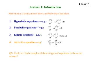
Class: 2. Lecture 1: Introduction. Mathematical Classification of Flows and Water Mass Equations. Hyperbolic equations-----e.g.: Parabolic equations----e.g.: Elliptic equations---e.g.: . Advective equation—e.g :.

Lecture 1: Introduction
E N D
Presentation Transcript
Class: 2 Lecture 1: Introduction Mathematical Classification of Flows and Water Mass Equations • Hyperbolic equations-----e.g.: • Parabolic equations----e.g.: • Elliptic equations---e.g.: . • Advective equation—e.g: QS. Could we find examples of these 4 types of equations in the ocean science?
Example for a hyperbolic equation: Oceanic waves Considering a 1-D linear surface gravity wave: Solving these 2 equations for : then, where
Example for a parabolic equation: Heat diffusion equation Then, we get Using the scaling analysis, we could find that the diffusion time scale is
Example for an elliptical equation: Pressure equation Solving for P, Then, we get
Example for an advective equation: Heat transport equation This means that the local change of the water temperature is caused by the replacement of water advected from upstream direction 20o 18o 16o 14o x u > 0
Classification of Discretization Methods • Finite-difference methods---Oldest methods • Finite-element methods----Popular in the last 10 years • Finite-volume methods---New Methods
FDM i i+1 x Difference between finite-difference, finite-element and finite-volume methods (FDM, FEM, and FVM) FEM FVM Integration Difference Variation
Advantage: Disadvantage: FDM FEM and FVM
Key Properties of Numerical Methods 1. Consistency Definition: The Discretization should approach the exact function as the discrete interval approach zero. F(x) Example: F(x4) F(x3) F(x5) Space interval: F(x1) F(x2) x x1 x2 x3 x4 x5... xn as
2. Stability Definition: A numerical method is defined to be stable if the numerical solution does not grow up an unreasonable big value or becomes infinite during the time integration. f(t) blows up ! o t Depending on: 1) time step/space resolution (linear), mass conservation and boundary conditions, etc Comments: A stable model does not means that is mass conservative.
Oscillation f(t) Exact value Convergence Non-convergence! t 3. Convergence A numerical method is defined to be convergent if the numerical solution of the discretization equation tends to reach the exact solution of the differential equation as grid spacing approaches zero.
4. Conservation The flow and water mass in the ocean follow the conservation laws. This means that in the absence of sources and sinks, the mass in local individual or global entire computational region should be conservative with a zero net flux into or out of the domain. • Finite-difference models: rectangular grids: conservative if specified care is made; • Finite-element models: Probably conservative over the entire domain but not individual element • Finite-volume models: Guarantee the mass conservation!
35 U > 0 0 x x 5. Boundedness For the realistic application, there are bounds for flows and water masses. For example, the turbulent kinetic energy always remains positive. Currents, temperature and salinity, etc should have a maximum and a minimum values in individual volume. Boundedness means here that numerical solution should be within these values. Examples: But the bounded minimum value is 0! Depends on 1) Computer round off; 2) Order of Approximation Comments: High order approximation scheme could easily cause the boundedness problem.
6. Realizability Many processes in the ocean are too complex to have an exact solution which, we believe, is absolutely correct. For example, no one could say that the MY 2.5 turbulence closure model is sufficiently enough to describe the turbulence in the ocean, though we found it works for many cases. A numerical method should be developed with caution in considering resolving the reality. Examples Tidal simulation: The time ramping. Similar: wind or other forcing.
7. Accuracy Once the equations are discretized and solved numerically, they only provided an approximate solution. The accuracy of this solution depends on grid resolution and the orders of the approximation. Examples: Coarse grids: low accuracy High order approximation: high accuracy but probably cause boundedness problems.