Download
1 / 17
170 likes | 307 Vues
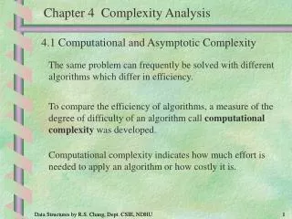
Chapter 4 Complexity Analysis. 4.1 Computational and Asymptotic Complexity. The same problem can frequently be solved with different algorithms which differ in efficiency.

E N D
Chapter 4 Complexity Analysis 4.1 Computational and Asymptotic Complexity The same problem can frequently be solved with different algorithms which differ in efficiency. To compare the efficiency of algorithms, a measure of the degree of difficulty of an algorithm call computational complexity was developed. Computational complexity indicates how much effort is needed to apply an algorithm or how costly it is. Data Structures by R.S. Chang, Dept. CSIE, NDHU 1
Chapter 4 Complexity Analysis 4.1 Computational and Asymptotic Complexity Time complexity: running time required (more important) Space complexity: memories required Time depends on: the algorithm, the machine used, the programming language used, the compiler used, the environment, the programming skill, etc.
Chapter 4 Complexity Analysis 4.1 Computational and Asymptotic Complexity To evaluate an algorithm’s efficiency, logical time units that express a relationship between the size n of an input and the amount of time t required to process the input should be used. t=f(n) Example: :輸入資料量增加一倍,執行時間增加一倍 :輸入資料量增加一倍,執行時間增加一
Chapter 4 Complexity Analysis 4.1 Computational and Asymptotic Complexity The resulting function gives only an approximate measure of efficiency. However, this approximation is sufficiently close, especially for a function which processes large quantities of data. The measure of efficiency is called asymptotic complexity and is used when disregarding certain terms of a function to express the efficiency of an algorithm.(只留函數中最重要的部分)
Chapter 4 Complexity Analysis 4.1 Computational and Asymptotic Complexity Example: Only the n2 term is important when n becomes large. Therefore, we say f(n)=O(n2)
Chapter 4 Complexity Analysis 4.2 Big-O Notation Definition: Given two positive-valued functions f and g, f(n) is O(g(n)) if there exist positive numbers c and N such that cg(n)f(n) for all nN. Example:
Chapter 4 Complexity Analysis 4.2 Big-O Notation • Problem with the big-O notation: • It states only that there must exist certain c and N, but it does not give any hint how to calculate these constants. • There can be infinitely many functions g for a given function f. For example, f(n)=O(n2)=O(n3)=O(n4)=... We want the lowest upper bound.
Chapter 4 Complexity Analysis 4.3 Properties of Big-O Notation Fact 1. (transitivity) If f(n) is O(g(n)) and g(n) is O(h(n)), then f(n) is O(h(n)). (i.e., f(n)=O(g(n))=O(O(h(n)))=O(h(n)). Fact 2. If f(n) is O(h(n)) and g(n) is O(h(n)) then f(n)+g(n) is O(h(n)). Fact 3. The function of ank is O(nk). Fact 4. The function nk is O(nk+j) for any positive j. Fact 5. If f(n)=cg(n) then f(n)=O(g(n)). Fact 6. logan=O(logbn) for any numbers a and b greater than 1. Fact 7. logan is O(log2n) for any positive a.
Chapter 4 Complexity Analysis 4.4 (omega) and (theta) Notations Definition 2. The function f is (g(n)) if there exist positive numbers c and N such that f(n)cg(n) for all nN. We want the greatest lower bound. f(n) is (g(n)) iff (if and only if) g(n) is O(f(n)).
Chapter 4 Complexity Analysis 4.4 (omega) and (theta) Notations Definition 3. f(n) is (g(n)) if there exist positive numbers c1, c2, and N such that c2g(n)f(n)c1g(n) for all nN. f(n) is (g(n)) iff f(n) is O(g(n)) and f(n) is (g(n)).
Chapter 4 Complexity Analysis 4.5 Possible Problems Big-O notation is the asymptotic complexity function. Please don’t forget there are concealed constants. For example: 108n is O(n) and 10n2 is O(n2). However, for 107n, 10n2 is better.
Chapter 4 Complexity Analysis 4.6 Examples of Complexities
Chapter 4 Complexity Analysis 4.6 Examples of Complexities
Chapter 4 Complexity Analysis 4.7 Finding Asymptotic Complexity: Examples Example 1: for (i=sum=0; i<n; i++) sum += a[i]; O(n) Example 2: for (i=0; i<n; i++) { for (j=1 sum=a[0]; j<=i; j++) sum += a[j]; printf(“sum for subarray 0 through %d is %d\n”,i,sum); }
Chapter 4 Complexity Analysis 4.7 Finding Asymptotic Complexity: Examples Example 3: for (i=4; i<n; i++) { for (j=i-3, sum=a[i-4]; j<=i; j++) sum += a[j]; printf(“sum for subarray %d through %d is %d\n”,i-4,i,sum); } O(n): 課本的計算式有誤
Chapter 4 Complexity Analysis 4.7 Finding Asymptotic Complexity: Examples Example 4: Determine the longest increasing subarray. For (I=0, length=1; I<n-1; I++) { for (i1=i2=k=I; k<n-1 && a[k]<a[k+1]; k++,i2++); if (length <i2-i1+1) length=i2-i1+1; } Worst case: O(n2) Best case: O(n) Average case: ???
Chapter 4 Complexity Analysis Exercise: 2 and 5 in Page 56.