Climate Modeling
Climate Modeling. Inez Fung University of California, Berkeley. Weather Prediction by Numerical Process Lewis Fry Richardson 1922. Weather Prediction by Numerical Process Lewis Fry Richardson 1922. Grid over domain Predict pressure, temperature, wind. Temperature -->density Pressure

Climate Modeling
E N D
Presentation Transcript
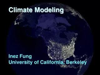
Climate Modeling Inez Fung University of California, Berkeley
Weather Prediction by Numerical ProcessLewis Fry Richardson 1922
Weather Prediction by Numerical ProcessLewis Fry Richardson 1922 • Grid over domain • Predict pressure, temperature, wind • Temperature • -->density • Pressure Pressure gradient • Wind • temperature
Weather Prediction by Numerical ProcessLewis Fry Richardson 1922 • Predicted: • 145 mb/ 6 hrs • Observed: • -1.0 mb / 6 hs
First Successful Numerical Weather Forecast: March 1950 • Grid over US • 24 hour, 48 hour forecast • 33 days to debug code and do the forecast • Led by J. Charney (far left) who figured out the quasi-geostrophic equations
ENIAC: <10 words of read/write memory Function tables (read memory)
16 operations in each time step Platzman, Bull. Am Meteorol. Soc. 1979
Reasons for success in 1950 • More & better observationsafter WWII--> initial conditions + assessment • Faster computers(24 hour forecast in 24 hours) • Improved physics - • Atm flow is quasi 2-D (Ro<<1) and is baroclinically unstable • quasi-geostrophic vorticity equations • filtered out gravity waves • Initial C: pressure (no need for u,v) • t ~30 minutes (instead of 5-10 minutes)
2007 Nobel Peace Prize toVP Al Gore andUN Intergovt Panel for Climate Change Bert Bolin 5/15/1925 - 12/30/2007 Founding Chairman of the IPCC … [student at 1950 ENIAC calculation]
Atmosphere momentum mass energy water vapor convective mixing
Ocean momentum mass energy salinity
Numerical Weather Prediction ( ~ days) Initial Conditions t = 0 hr Prediction t = 6 hr 12 18 24 • Predict evolution of state of atmosphere (t) • Error grows w time --> limit to weather prediction
Seasonal Climate Prediction ( El – Nino Southern Oscillation ) {Prediction} t = 1 month 2 3 { Initial Conditions} Atm + Ocn t = 0 • Coupled atmosphere-ocean instability • Require obs of initial states of both atm & ocean, • esp. Equatorial Pacific • {Ensemble} of forecasts • Forecast statistics (mean & variance) – probability • Now – experimental forecasts (model testing in ~months)
Continued Success Since 1950 • More & better observations • Faster computers • Improved physics
Modern climate models • Forcing:solar irradiance, volanic aerosols, greenhouse gases, … • Predict:T, p, wind, clouds, water vapor, soil moisture, ocean current, salinity, sea ice, … • Very high spatial resolution: • <1 deg lat/lon resolution • ~50 atm, ~30 ocn, ~10 soil layers • ==> 6.5 million grid boxes • Very small time steps(~minutes) • Ensemble runsmultiple experiments) • Model experiments (e.g. 1800-2100) take weeks to months on supercomputers
Continued Success Since 1950 • More & better observations • Faster computers • Improved physics
Earth’s Energy Balance, with GHG Sun Earth 100 70 30 20absorbed by atm 23 7 114 95 CO2, H2O, GHG 50 absorbed by sfc
Climate Processes • Radiative transfer: solar & terrestrial • phase transition of water • Convective mixing • cloud microphysics • Evapotranspirat’n • Movement of heat and water in soils
Climate Forcing CO2 change in radiative heating (W/m2) at surface for a given change in trace gas composition or other change external to the climate system CH4 N2O 10,000 years ago
Climate Feedbacks Decrease snow cover; Decrease reflectivity of surface Increase absorption of solar energy Evaporation from ocean, Increase water vapor in atm Enhance greenhouse effect Increase cloud cover; Decrease absorption of solar energy Warming
Urgency: Rapid Melting of Glaciers --> accelerate warming J. Zwally Moulin Greenland
Will cloud cover increase or decrease with warming? [models: decrease; warm air can hold more moisture; +ve feedback] Saturation Vapor Pressure (mb) Temperature (K) C A B + water vapor + longwave abs Warming liquid B A C + water vapor + cloud cover + longwave abs - shortwave abs A vapor 275 280 285 290 295 300
Attribution Observations • are observed changes consistent with • expected responses to forcings • inconsistent with alternative explanations Climate model: All forcing Climate model: Solar+volcanic only IPCC AR4 (2007)
Oceans: Bottleneck to warminglong memory of climate system • 4000 meters of water, heated from above • Stably stratified • Very slow diffusion of chemicals and heat to deep ocean • Fossil fuel CO2: • 200 years emission, • penetrated to upper 500-1000 m • Slow warming of oceans --> continue evaporation, continue warming
21stC warming depends on rate of CO2 increase 21thC “Business as usual”: CO2 increasing 380 to 680 ppmv 20thC stabilizn: CO2 constant at 380 ppmv for the 21stC Meehl et al. (Science 2005)
Model predicted change in recurrence of “100 year drought” 2020s 2070s years Changes in the probability distribution as well the mean
Outlook • More & better observations • Faster computers • Improved physics + Biogeochemistry: include atmospheric chemistry, land and ocean biology to predict climate forcing and surface boundary conditions
Atmosphere momentum mass energy water vapor convective mixing
Ship Tracks:- more cloud condensation nuclei- smaller drops- more drops- more reflective- D energy balance
Climate Model’s View of the Global C Cycle Atmosphere CO2 = 280 ppmv (560 PgC) + … 90± 60± Turnover Time of C 102-103 yr Turnover time of C 101yr Ocean Circ. + BGC 2000 Pg C 37400 Pg C Biophysics + BGC FF
Prognostic Carbon Cycle Atm Ocean Land-live Land-dead
21st C Carbon-Climate Feedback: = Coupled minus Uncoupled {dT, Soil Moisture Index} Warm-wet Warm-dry Regression of NPP vs T Photosynthesis decreases with carbon-climate coupling Fung et al. Evolution of carbon sinks in a changing climate. PNAS 2005
Changing Carbon Sink Capacity CO2 Airborne fraction =atm increase / Fossil fuel emission • With SRES A2 (fast FF emission): as CO2 increases • Capacity of land and ocean to store carbon decreases (slowing of photosyn; reduce soil C turnover time; slower thermocline mixing …) • Airborne fraction increases --> more warming Fung et al. Evolution of carbon sinks in a changing climate. PNAS 2005
Continued Success Since 1950 • More & better observations: • initial conditions, • Analysis --> improve physics • assessment of model results • Faster computers • Improved physics
Initial Condition: Numerical Weather Prediction Challenge Diverse, asynchronous obs of atm Find the current state of the atm at tn Model --> forecast for tn+1 Practice Ensemble forecast --> mean state, uncertainty in forecast Kalnay 2003
Approach: Data Assimilation obs yo yo xa Model: xbn= M(xan-1) xb tn-1 tn Find best estimate of x (xan) given imperfect model (xbn) and incomplete obs (yo) x=[T, p, u,v, q, s, … model parameters] yo
Approaches to Merge Data + Model • Optimal analysis • 3D variational data assimilation • 4D var • Kalman Filter • Ensemble Kalman Filter • Local Ensemble Transform Kalman Filter • …
Observations: The A-Train 4/28/2006 Coordinated Observations 5/4/2002 12/18/2004 1:26 CloudSat – 3-D cloud climatology CALIPSO – 3-D aerosol climatology 7/15/2004 aerosols, polarization AIRS – T, P, H2O, CO2, CH4 MODIS – cloud, aerosols, albedo TES – T, P, H2O, O3, CH4, CO MLS – O3, H2O, CO HIRDLS – T, O3, H2O, CO2, CH4 OMI – O3, aerosol climatology OCO - - CO2 O2 A-band ps, clouds, aerosols Challenge: assimilating ALL data simultaneously in high-resolution climate model to understand interactions
Outlook: Research challenges • Climate Change Science: • High resolution climate projections 1800-2030: • Project impact on water availability, ecosystems, agriculture, at a resolution useful to inform policy and strategies for adaptation and carbon management • Articulation of uncertainties and risks
Outlook: Research challenges Adaptation and Mitigation • Production and consumption energy efficiency • Alternative energy • Carbon capture & sequestrat’n - scalable? • Geo-engineering - potential harm vs benefits Maturity Need a new generation of models where climate interacts with adaptation and mitigation strategies to guide, prioritize policy decisions
http://www.ipcc.ch 4th Assessment Report 2007 WGI: Science WGII: Impacts WGIII: Adaptation and Mitigation