The “Humpty Dumpty” problem
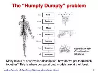
The “Humpty Dumpty” problem. figure taken from Churchland and Sejnowski. Many levels of observation/description: how do we get them back together? This is where computational models are at their best. Prelude: Self-Organization. genome: ~10 9 bits brain: ~10 15 connections

The “Humpty Dumpty” problem
E N D
Presentation Transcript
The “Humpty Dumpty” problem figure taken from Churchland and Sejnowski Many levels of observation/description: how do we get them back together? This is where computational models are at their best.
Prelude: Self-Organization • genome: ~109 bits • brain: ~1015 connections • → thus, genome can’t explicitly code wiring pattern of brain • Where does pattern come from? • some through learning from external inputs • but a lot of structure seems to develop before sensory input • has a chance to shape the system • Where does structure come from?
Self-Organization: “structure for free” figures taken from Haken “street” patterns in clouds presence of water droplets facilitates condensation of more vapour
figure taken from Haken wave pattern in chemical reaction presence of one reaction product catalyzes production of others
Benard system figures taken from Kelso presence of one convection cell stabilizes presence of its neighbors
Social insects: termite mounds activity of one termite encourages others to “follow its path” http://iridia.ulb.ac.be/~mdorigo/ACO/RealAnts.html
Principles of Self-Organization • In all the examples: • structure emerges from interactions of simple components • in general, three ingredients: • positive feedback loops (self-amplification) • cooperation between some elements • limited resources: competition between elements Let’s keep looking for these…
Organizing Principles for Learning in the Brain Associative Learning: Hebb rule and variations, self-organizing maps Adaptive Hedonism: Brain seeks pleasure and avoids pain: conditioning and reinforcement learning Imitation: Brain specially set up to learn from other brains? Imitation learning approaches Supervised Learning: Of course brain has no explicit teacher, but timing of development may lead to some circuits being trained by others
Unsupervised Hebbian Learning Idea: (D. Hebb, 1948?) Strengthening of connections between coactive units. physiological basis of Hebbian learning: Long Term Potentiation (LTP) figure taken from Dayan&Abbott
Spike timing dependent plasticity (STDP): temporal fine structure of correlations may be crucial! Synapse strengthened if pre-synaptic spike predicts post-synaptic spike figure taken from Dayan&Abbott
connection weights activity patterns Network Self-organization Recall our 3 ingredients: - positive feedback loops (self-amplification) - cooperation between some elements - limited resources: competition between elements A C B • correlated activity leads to weight growth (Hebb) • weight growth leads to more correlated activity • weight growth limited due to competition
Single linear unit with simple Hebbian learning figure taken from Hertz et.al. one of the simplest model neurons • Simple Hebbian learning: • η is learning rate • inputs draw from some probability distribution • simple Hebb rule moves weight vector in direction of current input • weight vector aligns with principal Eigenvector of input correlation matrix • Problem: weights can grow without bounds, need competition
Excursion: Correlation and Covariance mean variance correlation matrix covariance matrix
Oja’s rule • Idea: subtract term proportional to V2 to limit weight growth • still leads to extraction of firstprincipal component of input correlation matrix Problem: don’t want weights to grow without bounds, i.e., “what comes up must go down”
Other “Hebbian” learning rules: • weight clipping • subtractive or multiplicative normalization • covariance rules extracting principal eigenvector of covariance matrix instead of correlation matrix • BCM rule (has some exp. support) • Yuille’s “non-local” rule, converges to Many, many ways to limit weight growth, sometimes very distinct differences in the learned weights!
correlation vs. covariance rules: figure taken from Dayan&Abbott
Multiple output units:Principal Component Analysis • Oja: • Sanger: Both rules give the first Eigenvectors of the correlation matrix
Retina Tectum Applications of Hebbian Learning:Retinotopic Connections Retinotopic: neighboring retina cells project to neighboring tectum cells, i.e. topology is preserved, hence “retinotopic” Question: How do retina units know where to project to? Answer: Retina axons find tectum through chemical markers, but fine structure of mapping is activity dependent
tectum x Retina Tectum tectum y simulation result: localized RFs in tectum Principal assumptions: - local excitation of neighbors in retina and tectum - Hebbian learning of feed-forward weights Hebbian learning models account for a wide range of experiments: half retina, half tectum, graft rotation, … half retina experiment
Applications of Hebbian Learning:Ocular Dominance • fixed lateral weights, • Hebbian learning of • feedforward weights, • exact form of weight • competition is very • important! figure taken from Dayan&Abbott Such models can qualitatively predict effects of blocking input from one eye, etc.
Applications of Hebbian Learning:Visual Receptive Field Formation figure taken from Dayan&Abbott more about these things next week!
Applications of Hebbian Learning:Visual Cortical Map Formation primary visual cortex: retinal position, ocular dominance, orientation selectivity all mapped onto 2-dim. map. Figure taken from Tanaka lab web page
ocularity retinal position move weight in direction of input move weight in direction of neighbors The Elastic Net Model Consider the different dimensions “retinal position”, “ocular dominance”, etc. as N scalar input dimensions. The selectivity of a unit a can be described by its position in a N-dimensional space. Its coordinates Wab are the preferred values along each dimension b. A unit’s activity is modeled with Gaussians: Learning rule:
Elastic Net Modeling Pinwheels simple elastic net model experiment learning rule moves units’ selectivities through ab- stract feature space optical im- aging study of V1 in macaque figure taken from Dayan&Abbott
Complex RF-LISSOM modelReceptive Field Laterally Interconnected Synergetically Self-Organizing Map Figures taken from http://www.cs.texas.edu/users/nn/web-pubs/htmlbook96/sirosh/
LISSOM Demo: learns feedforward and lateral weights, inputs are elongated blobs (simulation needs power of supercomputer)
Summary: Hebbian Learning Modelsin Development • There are many, many ways of modeling Hebbian learning: correlation & covariance based, timing dependent, etc. • Different kinds of Hebbian learning models at different levels of abstraction have been applied to modeling some developmental phenomena, e.g.: • emergence of retinotopic connections • development of ocular dominance • emergence of visual receptive fields • cortical map formation • Typically, the inputs of the network are assumed to have simple static distribution. Hardly any work on learning agents that interact with their environment and influence statistics of their sensory input (recall the kitten experiments we read about).
Four questions to discuss/think about • Different levels of abstraction, e.g., compartmental, spiking point neurons learning with STDP, or simple model of rate coding neuron, abstract SOM like models; what is the right level of abstraction? • Even at one level of abstraction there are many different “Hebbian” learning rules; is it important which one you use? What is the right one? • The applications we discussed considered networks passively receiving sensory input and learning to code it; how can we model learning through interaction with environment? Why might it be important to do so? • The problems we considered so far are very “low-level”, no hint of “behaviors” (like that observed in an infant preferential looking task) yet. How can we bridge this huge divide?