Chapter 6. Residues and Poles

1. Chapter 6. Residues and Poles Weiqi Luo (骆伟祺) School of Software Sun Yat-Sen University Email：weiqi.luo@yahoo.com Office：# A313

2. Chapter 6: Residues and Poles • Isolated Singular Points • Residues • Cauchy’s Residue Theorem • Residue at Infinity • The Three Types of Isolated Singular Points • Residues at Poles; Examples • Zeros of Analytic Functions; • Zeros and Poles • Behavior of Functions Near Isolated singular Points

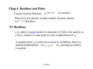
3. 68. Isolated Singular Points • Singular Point A point z0 is called a singular point of a function f if f fails to be analytic at z0 but is analytic at some point in every neighborhood of z0. • Isolated Singular Point A singular point z0 is said to be isolated if, in addition, there is a deleted neighborhood 0<|z-z0|<ε of z0 throughout which f is analytic.

4. y y y ε ε ε ε x x x x 68. Isolated Singular Points • Example 1 The function has the three isolated singular point z=0 and z=±i. • Example 2 The origin is a singular point of the principal branch Not Isolated.

5. 68. Isolated Singular Points • Example 3 The function has the singular points z=0 and z=1/n (n=±1,±2,…), all lying on the segment of the real axis from z=-1 to z=1. Each singular point except z=0 is isolated.

6. 68. Isolated Singular Points • If a function is analytic everywhere inside a simple closed contour C except a finite number of singular points : z1, z2, …, zn then those points must all be isolatedand the deleted neighborhoods about them can be made small enough to lie entirely inside C. • Isolated Singular Point at ∞ If there is a positive number R1 such that f is analytic for R1<|z|<∞, then f is said to have an isolated singular point at z0=∞.

7. 69. Residues • Residues When z0 is an isolated singular point of a function f, there is a positive number R2 such that f is analytic at each point z for which 0<|z-z0|<R2. then f(z) has a Laurent series representation where the coefficients an and bn have certain integral representations. where C is any positively oriented simple closed contour around z0 hat lies in the punctured disk 0<|z-z0|<R2. Refer to pp.198

8. 69. Residues • Residues (Cont’) Then the complex number b1 is called the residues of f at the isolated singular point z0, denoted as

9. 69. Residues • Example 1 Consider the integral where C is the positively oriented unit circle |z|=1. Since the integrand is analytic everywhere in the finite plane except z=0, it has a Laurent series representation that is valid when 0<|z|<∞.

10. 69. Residues • Example 1 (Cont’)

11. 69. Residues • Example 2 Let us show that when C is the same oriented circle |z|=1. Since the 1/z2 is analytic everywhere except at the origin, the same is true of the integrand. One can write the Laurent series expansion

12. 69. Residues • Example 3 A residues can also be used to evaluate the integral where C is the positively oriented circle |z-2|=1. Since the integrand is analytic everywhere in the finite plane except at the point z=0 and z=2. It has a Laurent series representation that is valid in the punctured disk

13. 69. Residues • Example 3 (Cont’)

14. 70. Cauchy’s Residue Theorem • Theorem Let C be a simple closed contour, described in the positive sense. If a function f is analytic inside and on C except for a finite number of singular points zk (k = 1, 2, . . . , n) inside C, then

15. 70. Cauchy’s Residue Theorem • Theorem (Cont’) Proof: Let the points zk (k=1,2,…n) be centers of positively oriented circles Ck which are interior to C and are so small that no two of them have points in common (possible?). Then f is analytic on all of these contours and throughout the multiply connected domain consisting of the points inside C and exterior to each Ck, then

16. 70. Cauchy’s Residue Theorem • Example Let us use the theorem to evaluate the integral

17. 70. Cauchy’s Residue Theorem • Example (Cont’) In this example, we can write

18. 71. Residue at Infinity • Definition Suppose a function f is analytic throughout the finite plane except for a finite number of singular points interior to a positively oriented simple close contour C. Let R1 is a positive number which is large enough that C lies inside the circle |z|=R1 The function f is evidently analytic throughout the domain R1<|z|<∞. Let C0 denote a circle |z|=R0, oriented in the clockwise direction, where R0>R1. The residue of f at infinity is defined by means of the equation

19. 71. Residue at Infinity Refer to the Corollary in pp.159 Based on the definition of the residue of f at infinity

20. 71. Residue at Infinity • Theorem If a function f is analytic everywhere in the finite plane except for a finite number of singular points interior to a positively oriented simple closed contour C, then

21. 71. Residue at Infinity • Example In the example in Sec. 70, we evaluated the integral of around the circle |z|=2, described counterclockwise, by finding the residues of f(z) at z=0 and z=1, since

22. 71. Homework • pp. 239-240 Ex. 2, Ex. 3, Ex. 5, Ex. 6

23. 72. The Three Types of Isolated Singular Points • Laurent Series If f has an isolated singular point z0, then it has a Laurent series representation In a punctured disk 0<|z-z0|<R2. is called the principal part of f at z0 In the following, we use the principal part to identify the isolated singular point z0 as one of three special types.

24. 72. The Three Types of Isolated Singular Points • Type #1: If the principal part of f at z0 at least one nonzero term but the number of such terms is only finite, the there exists a positive integer m (m≥1) such that and Where bm ≠ 0, In this case, the isolated singular point z0 is called a pole of order m. A pole of order m=1 is usually referred to as a simple pole.

25. 72. The Three Types of Isolated Singular Points • Example 1 Observe that the function has a simple pole (m=1) at z0=2. It residue b1 there is 3.

26. 72. The Three Types of Isolated Singular Points • Example 2 From the representation One can see that f has a pole of order m=2 at the origin and that

27. 72. The Three Types of Isolated Singular Points • Type #2 If the principal part of f at z0 has no nonzero term z0 is known as a removable singular point, and the residues at a removable singular point is always zero. Note: f is analytic at z0 when it is assigned the value a0 there. The singularity z0 is, therefore, removed.

28. 72. The Three Types of Isolated Singular Points • Example 4 The point z0=0 is a removable singular point of the function Since when the value f(0)=1/2 is assigned, f becomes entire.

29. 72. The Three Types of Isolated Singular Points • Type #3 If the principal part of f at z0 has infinite number of nonzero terms, and z0 is said to be an essential singular point of f. • Example 3 Consider the function has an essential singular point at z0=0. where the residue b1 is 1.

30. 72. Homework • pp. 243 Ex. 1, Ex. 2, Ex. 3

31. 73. Residues at Poles • Theorem An isolated singular point z0 of a function f is a pole of order m if and only if f (z) can be written in the form where φ(z) is analytic and nonzero at z0 . Moreover,

32. 73. Residues at Poles • Proof the Theorem Assume f(z) has the following form where φ(z) is analytic and nonzero at z0, then it has Taylor series representation b1 a pole of order m, φ(z0)≠0

33. 73. Residues at Poles On the other hand, suppose that The function φ(z) defined by means of the equations Evidently has the power series representation Throughout the entire disk |z-z0|<R2. Consequently, φ(z) is analytic in that disk, and, in particular, at z0. Here φ(z0) = bm≠0.

34. 74. Examples • Example 1 The function has an isolated singular point at z=3i and can be written Since φ(z) is analytic at z=3i and φ(3i)≠0, that point is a simple pole of the function f, and the residue there is The point z=-3i is also a simple pole of f, with residue B2= 3+i/6

35. 74. Examples • Example 2 If then The function φ(z) is entire, and φ(i)=i ≠0. Hence f has a pole of order 3 at z=i, with residue

36. 74. Examples • Example 3 Suppose that where the branch find the residue of f at the singularity z=i. The function φ(z) is analytic at z=i, and φ(i)≠0, thus f has a simple pole there, the residue is B= φ(i)=-π3/16.

37. 74. Examples • Example 5 Since z(ez-1) is entire and its zeros are z=2nπi, (n=0, ±1, ±2,… ) the point z=0 is clearly an isolated singular point of the function From the Maclaurin series We see that Thus

38. 74. Examples • Example 5(Cont’) since φ(z) is analytic at z=0 and φ(0) =1≠0, the point z=0 is a pole of the second order. Thus, the residue is B= φ’(0) Then B=-1/2.

39. 74. Examples • pp. 248 Ex. 1, Ex. 3, Ex. 6

40. 75. Zeros of Analytic Functions • Definition Suppose that a function f is analytic at a point z0. We known that all of the derivatives f(n)(z0) (n=1,2,…) exist at z0. If f(z0)=0 and if there is a positive integer m such that f(m)(z0)≠0 and each derivative of lower order vanishes at z0, then f is said to have a zero of order m at z0.

41. 75. Zeros of Analytic Functions • Theorem 1 Let a function f be analytic at a point z0. It has a zero of order m at z0 if and only if there is a function g, which is analytic and nonzero at z0 , such that Proof: • Assume that f(z)=(z-z0)mg(z) holds, Note that g(z) is analytics at z0, it has a Taylor series representation

42. 75. Zeros of Analytic Functions Thus f is analytic at z0, and Hence z0 is zero of order m of f. 2) Conversely, if we assume that f has a zero of order m at z0, then g(z)

43. 75. Zeros of Analytic Functions The convergence of this series when |z-z0|<ε ensures that g is analytic in that neighborhood and, in particular, at z0, Moreover, This completes the proof of the theorem.

44. 75. Zeros of Analytic Functions • Example 1 The polynomial has a zero of order m=1 at z0=2 since where and because f and g are entire and g(2)=12≠0. Note how the fact that z0=2 is a zero of order m=1 of f also follows from the observations that f is entire and that f(2)=0 and f’(2)=12≠0.

45. 75. Zeros of Analytic Functions • Example 2 The entire function has a zero of order m=2 at the point z0=0 since In this case,

46. 75. Zeros of Analytic Functions • Theorem 2 Given a function f and a point z0, suppose that • f is analytic at z0 ; • f (z0) = 0 but f (z) is not identically equal to zero in any neighborhood of z0. Then f (z) ≠ 0 throughout some deleted neighborhood 0 < |z − z0| < ε of z0.

47. 75. Zeros of Analytic Functions Proof: Since (a) f is analytic at z0, (b) f (z0) = 0 but f (z) is not identically equal to zero in any neighborhood of z0 , f must have a zero of some finite order m at z0(why?).According to Theorem 1, then where g(z) is analytic and nonzero at z0. Since g(z0)≠0 and g is continuous at z0, there is some neighborhood |z-z0|<ε, g(z) ≠0. Consequently, f(z) ≠0 in the deleted neighborhood 0<|z-z0|<ε (why?)

48. 75. Zeros of Analytic Functions • Theorem 3 Given a function f and a point z0, suppose that • f is analytic throughout a neighborhood N0 of z0 • f (z) = 0 at each point z of a domain D or line segment L containing z0. Then in N0 That is, f(z) is identically equal to zero throughout N0

49. 75. Zeros of Analytic Functions Proof: We begin the proof with the observation that under the stated conditions, f (z) ≡ 0 in some neighborhood N of z0. For, otherwise, there would be a deleted neighborhood of z0 throughout which f(z)≠0, according to Theorem 2; and that would be inconsistent with the condition that f(z)=0 everywhere in a domain D or on a line segment L containing z0. Since f (z) ≡ 0 in the neighborhood N, then, it follows that all of the coefficients in the Taylor series for f (z) about z0 must be zero.

50. 75. Zeros of Analytic Functions • Lemma (pp.83) Suppose that • a function f is analytic throughout a domain D; • f (z) = 0 at each point z of a domain or line segment contained in D. Then f (z) ≡ 0 in D; that is, f (z) is identically equal to zero throughout D.