Multivariate Twin Analysis Matrix Raw Data Script
This script conducts multivariate twin analysis using matrix raw data to estimate cross-twin correlations and trait correlations. It explores genetic and environmental influences on family functioning and happiness.

Multivariate Twin Analysis Matrix Raw Data Script
E N D
Presentation Transcript
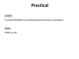
Practical SCRIPT: F:\meike\2010\Multi_prac\MultivariateTwinAnalysis_MatrixRaw.r DATA: DHBQ_bs.dat
DATA - General Family Functioning, Subjective Happiness - T1, T2, brother, sister - missing -999
DATA require(OpenMx) source("GenEpiHelperFunctions.R") FamData <- read.table (“DHBQ_bs.dat", header=T, na=-999) require(psych) summary (FamData) describe(FamData) names(FamData) Famvars <- colnames (FamData) Vars <- c('gff', 'hap') nv <- 2 selVars <- paste(Vars,c(rep(1,nv),rep(2,nv)),sep="") #c('gff1', 'hap1','gff2' 'hap2') ntv <- nv*2 mzData <- subset(FamData, zyg2==1, selVars) dzData <- subset(FamData, zyg2==2, selVars)
Observed Cross-twin Cross-trait Correlations # Print Descriptives summary(mzData) summary(dzData) describe(mzData) describe(dzData) colMeans(mzData,na.rm=TRUE) colMeans(dzData,na.rm=TRUE) cov(mzData,use="complete") cov(dzData,use="complete") cor(mzData,use="complete") cor(dzData,use="complete")
Observed Cross-twin Cross-trait Correlations > cor(mzData,use="complete") gff1 hap1 gff2 hap2 gff1 1.00 0.40 0.50 0.27 hap1 0.40 1.0 0.26 0.31 gff2 0.50 0.26 1.00 0.31 hap2 0.27 0.31 0.31 1.00 > cor(dzData,use="complete") gff1 hap1 gff2 hap2 gff1 1.00 0.35 0.35 0.12 hap1 0.35 1.00 0.19 0.15 gff2 0.35 0.19 1.00 0.32 hap2 0.12 0.15 0.32 1.00 >
Estimated Cross-twin Cross-trait Correlations # Fit Model to estimate Twin Correlations and Cross-twin Cross trait correlations by ML multTwinCorModel <- mxModel(multTwinSatFit, name="multTwinSatCor", mxModel(multTwinSatFit$MZ, mxMatrix( type="Iden", nrow=ntv, ncol=ntv, name="I"), mxAlgebra( expression= solve(sqrt(I*expCovMZ)) %*% expCovMZ %*% solve(sqrt(I*expCovMZ)), name="expCorMZ" ) ), mxModel(multTwinSatFit$DZ, mxMatrix( type="Iden", nrow=ntv, ncol=ntv, name="I"), mxAlgebra( expression= solve(sqrt(I*expCovDZ)) %*% expCovDZ %*% solve(sqrt(I*expCovDZ)), name="expCorDZ" ) ) ) multTwinCorFit <- mxRun(multTwinCorModel) multTwinCorFit$MZ$expCorMZ multTwinCorFit$DZ$expCorDZ
PRAC I.Estimated Cross-twin Cross-trait Correlations 1. Run Script 2. Compare Observed and Estimated Cross-Twin Cross-Trait Correlations 3. Based on these correlations what do you expect for A, C, and E (var and cov!)?
Cross-twin Cross-trait Correlations Within individual cross trait correlation Twin correlations Cross-twin cross-trait correlations > cor(mzData,use="complete") gff1 hap1 gff2 hap2 gff1 1.00 0.40 0.50 0.27 hap1 0.40 1.0 0.26 0.31 gff2 0.50 0.26 1.00 0.31 hap2 0.27 0.31 0.31 1.00 > cor(dzData,use="complete") gff1 hap1 gff2 hap2 gff1 1.00 0.35 0.35 0.12 hap1 0.35 1.00 0.19 0.15 gff2 0.35 0.19 1.00 0.32 hap2 0.12 0.15 0.32 1.00 > mxAlgebra 'expCorMZ' [,1] [,2] [,3] [,4] [1,] 1.00 0.38 0.48 0.25 [2,] 0.38 1.00 0.24 0.29 [3,] 0.48 0.24 1.00 0.30 [4,] 0.25 0.29 0.30 1.00 mxAlgebra 'expCorDZ' [,1] [,2] [,3] [,4] [1,] 1.00 0.35 0.36 0.13 [2,] 0.35 1.00 0.20 0.16 [3,] 0.36 0.20 1.00 0.34 [4,] 0.13 0.16 0.34 1.00
ACE model GFF --> MZ > DZ, but not >2x -> ACE HAP--> MZ > DZ-> ACE, AE GFF-HAP --> MZ > DZ-> ACE, AE Start with an ACE model
PRAC II.The ACE model and its estimates 1. Run the ACE model 2. What is the heritability of GFF and HAP? 3. What is the genetic influence on the covariance? 4. What is the genetic correlation?
Standardized Variance and Covariance Components [1] "Matrix ACE.A/ACE.V" stCovComp_A1 stCovComp_A2 gff 0.2491 0.4784 hap 0.4784 0.2673 [1] "Matrix ACE.C/ACE.V" stCovComp_C1 stCovComp_C2 gff 0.2441 0.2417 hap 0.2417 0.0292 [1] "Matrix ACE.E/ACE.V" stCovComp_E1 stCovComp_E2 gff 0.5069 0.2799 hap 0.2799 0.7035 GFF --> MZ > DZ, but not >2x -> ACE HAP--> MZ > DZ-> ACE, AE GFF-HAP --> MZ > DZ-> ACE, AE
Genetic and Environmental Correlations [1] "Matrix solve(sqrt(ACE.I*ACE.A)) %*% ACE.A %*% solve(sqrt(ACE.I*ACE.A))" corComp_A1 corComp_A2 gff 1.0000 0.6477 hap 0.6477 1.0000 [1] "Matrix solve(sqrt(ACE.I*ACE.C)) %*% ACE.C %*% solve(sqrt(ACE.I*ACE.C))" corComp_C1 corComp_C2 gff 1.0000 1.0000 hap 1.0000 1.0000 [1] "Matrix solve(sqrt(ACE.I*ACE.E)) %*% ACE.E %*% solve(sqrt(ACE.I*ACE.E))" corComp_E1 corComp_E2 gff 1.0000 0.1637 hap 0.1637 1.0000 >
ACE vs AE model # Fit Multivariate AE model # ----------------------------------------------------------------------- multAEModel <- mxModel(multACEFit, name="multAE", mxModel(multACEFit$ACE, mxMatrix( type="Lower", nrow=nv, ncol=nv, free=FALSE, values=0, name="c" ) # drop c at 0 ) ) > tableFitStatistics(multACEFit, multAEFit) Name ep -2LL df AIC diffLL diffdf p Model 1 : multACE 11 61033.46 10426 40181.46 - - - Model 2 : multAE 8 61058.94 10429 40200.94 25.49 3 0
Standardized Variance and Covariance Components [1] "Matrix ACE.A/ACE.V" stCovComp_A1 stCovComp_A2 gff 0.2491 0.4784 hap 0.4784 0.2673 [1] "Matrix ACE.C/ACE.V" stCovComp_C1 stCovComp_C2 gff 0.2441 0.2417 hap 0.2417 0.0292 [1] "Matrix ACE.E/ACE.V" stCovComp_E1 stCovComp_E2 gff 0.5069 0.2799 hap 0.2799 0.7035
ACE vs ACEAE model # Fit Multivariate GFF-ACE & HAP-AE model # ----------------------------------------------------------------------- multACE_ACEAEModel <- mxModel(multACEFit, name="multACE_ACEAE", mxModel(multACEFit$ACE, mxMatrix( type="Lower", nrow=nv, ncol=nv, free=c(T,F,F), values=0, name="c" ) # drop c21 & c22 at 0 ) ) Name ep -2LL df AIC diffLL diffdf p Model 1 : multACE 11 61033.46 10426 40181.46 - - - Model 2 : multAE 8 61058.94 10429 40200.94 25.49 3 0 Model 3 : multACE_ACEAE 9 61037.98 10428 40181.98 4.53 2 0.1
Genetic and Environmental Correlations [1] "Matrix solve(sqrt(ACE.I*ACE.A)) %*% ACE.A %*% solve(sqrt(ACE.I*ACE.A))" corComp_A1 corComp_A2 gff 1.0000 0.6477 hap 0.6477 1.0000 [1] "Matrix solve(sqrt(ACE.I*ACE.C)) %*% ACE.C %*% solve(sqrt(ACE.I*ACE.C))" corComp_C1 corComp_C2 gff 1.0000 1.0000 hap 1.0000 1.0000 [1] "Matrix solve(sqrt(ACE.I*ACE.E)) %*% ACE.E %*% solve(sqrt(ACE.I*ACE.E))" corComp_E1 corComp_E2 gff 1.0000 0.1637 hap 0.1637 1.0000 > Is the .65 significant different from 1 ?
rA=1 multACE_AcModel <- mxModel(multACEFit, name="multACE_Ac", mxModel(multACEFit$ACE, mxMatrix( type="Lower", nrow=nv, ncol=nv, free=c(T,T,F), values=0, name="a" ) # drop a22 at 0 ) ) Name ep -2LL df AIC diffLL diffdf p Model 1 : multACE 11 61033.46 10426 40181.46 - - - Model 2 : multAE 8 61058.94 10429 40200.94 25.49 3 0 Model 3 : multACE_ACEAE 9 61037.98 10428 40181.98 4.53 2 0.1 Model 4 : multACE_Ac 10 61036.73 10427 40182.73 3.27 1 0.07 Model 5 : multBest 8 61038.61 10429 40180.61 5.15 3 0.16
PRAC III.Trivariate Model 1. Add a third variable (Satisfaction with Life) to the model 2. Run model and submodels 3. What is the best fitting model? 2. What are the parameter estimates? 3. What is the genetic correlation?
Changes that had to be made FamData <- read.table ("DHBQ_bs.dat", header=T, na=-999) require(psych) summary (FamData) describe(FamData) names(FamData) Famvars <- colnames (FamData) Vars <- c('gff', 'hap', 'sat') nv <- 3 selVars <- paste(Vars,c(rep(1,nv),rep(2,nv)),sep="") #c('gff1', 'hap1', 'sat1','gff2' 'hap2', 'sat2') ntv <- nv*2 mzData <- subset(FamData, zyg2==1, selVars) dzData <- subset(FamData, zyg2==2, selVars)
Changes that had to be made multACEModel <- mxModel("multACE", mxModel("ACE", # Matrices a, c, and e to store a, c, and e path coefficients mxMatrix( type="Lower", nrow=nv, ncol=nv, free=TRUE, values=.6, label=c("a11", "a21", "a31", "a22", "a32", "a33"), name="a" ), mxMatrix( type="Lower", nrow=nv, ncol=nv, free=TRUE, values=.6, label=c("c11", "c21", "c31", "c22", "c32", "c33"), name="c" ), mxMatrix( type="Lower", nrow=nv, ncol=nv, free=TRUE, values=.6, label=c("e11", "e21", "e31", "e22", "e32", "e33"), name="e" ),
Changes that had to be made # Fit Multivariate ACE-AE-AE model # ----------------------------------------------------------------------- multACEAEAEModel <- mxModel(multACEFit, name="multACEAEAE", mxModel(multACEFit$ACE, mxMatrix( type="Lower", nrow=nv, ncol=nv, free=c(T,F,F,F,F,F), values=c(.5,0,0,0,0,0),, name="c" ) ) )
Changes that had to be made # Fit Multivariate ACE-AE-AE model # ----------------------------------------------------------------------- multACEAEAEModel <- mxModel(multACEFit, name="multACEAEAE", mxModel(multACEFit$ACE, mxMatrix( type="Lower", nrow=nv, ncol=nv, free=c(T,F,F,F,F,F), values=c(.5,0,0,0,0,0),, name="c" ) ) )
Genetic and Environmental Influences [1] "Matrix ACE.A/ACE.V" stCovComp_A1 stCovComp_A2 stCovComp_A3 gff 0.2882 0.7759 0.8403 hap 0.7759 0.3027 0.3973 sat 0.8403 0.3973 0.3854 [1] "Matrix ACE.C/ACE.V" stCovComp_C1 stCovComp_C2 stCovComp_C3 gff 0.2066 0.0000 0.0000 hap 0.0000 0.0000 0.0000 sat 0.0000 0.0000 0.0000 [1] "Matrix ACE.E/ACE.V" stCovComp_E1 stCovComp_E2 stCovComp_E3 gff 0.5052 0.2241 0.1597 hap 0.2241 0.6973 0.6027 sat 0.1597 0.6027 0.6146
Genetic and Environmental Correlations [1] "Matrix solve(sqrt(ACE.I*ACE.A)) %*% ACE.A %*% solve(sqrt(ACE.I*ACE.A))" corComp_A1 corComp_A2 corComp_A3 gff 1.0000 0.9014 0.9139 hap 0.9014 1.0000 0.8410 sat 0.9139 0.8410 1.0000 [1] "Matrix solve(sqrt(ACE.I*ACE.E)) %*% ACE.E %*% solve(sqrt(ACE.I*ACE.E))" corComp_E1 corComp_E2 corComp_E3 gff 1.0000 0.1295 0.1039 hap 0.1295 1.0000 0.6654 sat 0.1039 0.6654 1.0000
After the Break Genetic and environmental factor analysis examples Common Pathway Model Independent Pathway Model