A Genetical Genomics Project
310 likes | 494 Vues
A Genetical Genomics Project. Richard Mott Wellcome Trust Centre for Human Genetics. Project Summary. Gene Expression Analysis Gene Coexpression Networks Comparison between tissues Comparison with phenotypes Gene Ontology Analysis

A Genetical Genomics Project
E N D
Presentation Transcript
A Genetical Genomics Project Richard Mott Wellcome Trust Centre for Human Genetics
Project Summary • Gene Expression Analysis • Gene Coexpression Networks • Comparison between tissues • Comparison with phenotypes • Gene Ontology Analysis • NB: There are many R packages available from CRAN for gene expression and network analysis, which are not covered in this lecture. • You should explore them!
Gene expression datasets • Hippocampus (460 mice), • Liver and Lung (260 mice) • 100 Phenotypes • Mice are from a Heterogeneous Stock, from 164 families
Gene Expression data • Gene expression measured on Illumina Mouse arrays • 47000 50-mer probes • Approx 2 probes per gene • Covariates (eg Sex, Family) also available • > load("liver.exp.RData") • > load("liver.cov.RData") • > source("expression.tutorial.R")
Exploring Expression Data > liver.median <- apply(liver.exp, 2, median ) > hist(liver.median, breaks=50) > liver.subset <- liver.exp[,liver.median>6]
Sex Effects • Which transcripts have different expression levels for the two sexes? • Use a T-test on each transcript • The R apply() function speeds up the analysis • First define a function tfunc that performs the T test and reports the P-value • tfunc <- function( X, GENDER ) { tt <- t.test( X ~ GENDER ); return(tt$p.value) } • Then compute the test for each transcript • > sex.pvalue <- apply(liver.subset, 2,tfunc, liver.cov$GENDER ) • Then plot the distribution of p-values • > hist( sex.pvalue, breaks=50) • >sum(sex.pvalue<1.0e-5) • [1] 78
Sex Effects 312/2796 (11%) of transcripts with median level > 6 have sex effects with P < 0.01 78/2796 (2%) of transcripts with median level > 6 have sex effects with P < 0.00001
Family effects (Heritability) • Which transcripts are affected by genetic background? • Use one-way ANOVA wrapped inside apply() • First define a function to return the p-value of the ANOVA: • anova.pvalue <- function( X, factor ) { • a <- anova(lm( X ~ factor)) • return(a[1,5]) • } • Then find the transcripts with high heritability • family <- apply( liver.subset, 2, anova.pvalue, liver.cov$Family )
Family Effects 18% of transcripts with median level >6 have heritability p-value < 0.01 0.2% of transcripts with median level >6 have heritability p-value < 0.00001
Body Weight • We can find transcripts associated with body weight in a similar fashion to family effects, except that linear regression is used. • Note that the direction of causality is no longer certain, ie it is not clear whether variation in a transcript is causative for variation in weight or vice versa > weight.pvalue <- apply( liver.subset, 2, anova.pvalue, liver.cov$EndNormalBW ) > hist(weight.pvalue,breaks=50)
Body Weight 11% of transcripts with median levels > 6 are significant at P < 0.01 1.5% of transcripts with median levels > 6 are significant at P < 0.00001
What do the genes do? • So far we have identified sets of genes which are associated with sex, family and weight • How can we characterise these genes ? • One popular method is to test if the annotations of these genes have unusual features. • Annotations include: • genome location • protein domain architecture (eg from INTERPRO) • gene function, where known (eg from GO) • From a statistical perspective, is is importation that a controlled vocabulary (ontology) is used to describe gene functions. • The analysis then does not have to understand any biology!!
The Gene Ontology (GO)http://www.geneontology.org/ • GO associates a set of GO-terms with every gene, describing aspects of the gene’s known function. • It has become a very popular tools for automated investigation of large sets of genes. • But note that: • GO is not complete, covering only biological processes, cellular components and molecular functions. Other ontologies are also important. • many genes have no known function
GO annotation Examples GO:0000001 mitochondrion inheritance GO:0000002 mitochondrial genome maintenance GO:0000003 reproduction GO:0000005 ribosomal chaperone activity GO:0000006 high affinity zinc uptake transporter activity GO:0000007 low-affinity zinc ion transporter activity GO:0000008 thioredoxin GO:0000009 alpha-1,6-mannosyltransferase activity GO:0000010 trans-hexaprenyltranstransferase activity GO:0000011 vacuole inheritance GO:0000012 single strand break repair ENSMUSG00000061404 Olfr936 GO:0001584 GO:0016020 GO:0007600 GO:0007166 GO:0004930 GO:0031224 GO:0003674 GO:0005623 GO:0050896 GO:0016021 GO:0004888 GO:0004871 GO:0050877 GO:0007582 GO:0005575 GO:0007186 GO:0007608 GO:0007165 GO:0004872 GO:0007154 GO:0044464 GO:0044425 GO:0004984 GO:0007606 GO:0050874 GO:0009987 GO:0051869 GO:0008150 ENSMUSG00000030105Arl8b GO:0016043 GO:0007046 GO:0051233 GO:0005737 GO:0016817 GO:0044424 GO:0048487 GO:0005515 GO:0016787 GO:0043014 GO:0005623 GO:0007028 GO:0044422 GO:0044237 GO:0007242 GO:0043228 GO:0005856 GO:0007582 GO:0008152 GO:0007165 GO:0015630 GO:0008092 GO:0019003 GO:0016462 GO:0005622 GO:0044464 GO:0007154 GO:0003824 GO:0006139 GO:0006364 GO:0005488 GO:0003924 GO:0043170 GO:0016818 GO:0019001 GO:0009987 GO:0005525 GO:0008150 GO:0017076 GO:0043229 GO:0006396 GO:0016072 GO:0007059 GO:0043232 GO:0050875 GO:0044430 GO:0043283 GO:0044446 GO:0030496 GO:0015631 GO:0003674 GO:0042254 GO:0007264 GO:0000166 GO:0005819 GO:0017111 GO:0044238 GO:0043226 GO:0016070 GO:0005575 GO:0006996 ENSMUSG00000042428Mgat3 GO:0016020 GO:0008375 GO:0043413 GO:0005615 GO:0044421 GO:0005737 GO:0031224 GO:0044267 GO:0044424 GO:0008194 GO:0009058 GO:0005623 GO:0044422 GO:0044237 GO:0007582 GO:0008152 GO:0044425 GO:0005622 GO:0044464 GO:0003824 GO:0044431 GO:0003830 GO:0043227 GO:0043170 GO:0019538 GO:0006487 GO:0009059 GO:0006412 GO:0009987 GO:0016740 GO:0008150 GO:0043229 GO:0006486 GO:0009101 GO:0050875 GO:0016758 GO:0043283 GO:0044446 GO:0005795 GO:0003674 GO:0009100 GO:0016021 GO:0005576 GO:0044238 GO:0044249 GO:0043226 GO:0043231 GO:0005575 GO:0044260 GO:0016757 GO:0006464 GO:0005794 GO:0043412GO:0044444
Testing for GO association • Set of genes G is classified into two groups eg by sex • A given GO annotation term classifies the genes into two groups (present, absent) • The data are a 2x2 contingency table classified by sex and GO, and the test of GO/sex association can be done either by a chi-squared test or by Fisher’s Exact Test FET, or a generalised linear model with Poisson link function. • The most popular methods use the FET, which can be calculated quickly using the hypergeometric distribution, and is exact even when the counts of data are small
Testing for GO association • Read in a file of mappings between Illumina probe ids and Ensembl Mouse gene ids transcripts <- read.delim("mouse.transcripts.genes.txt", h=T) • Match them to the expressed transcripts (note that not all transcripts match genes) idx <- match( colnames(liver.exp), transcripts$transcript) > length(idx) [1] 47429 > sum(is.na(idx)) [1] 9343 • Read in a file of GO terms associated with each Ensembl Mouse gene (this set has been reduced to include only those GO terms present in more than 5% of genes) • go1 <- read.delim("GO.Ensembl.01.txt") • > dim(go1) • [1] 19988 387
Testing for GO association • Find the common transcripts between liver.subset and the annotations, and those transcripts with sex p-values < 0.01 > intersect <- colnames(liver.subset)[match(go1$transcript, colnames(liver.subset), nomatch = 0)] > intersect <- unique(sort(intersect)) > liver.subset.intersect <- liver.subset[, match(intersect, colnames(liver.subset))] > dim( liver.subset.intersect) [1] 275 1650 > go.intersect <- go1[match(intersect,go1$transcript),] > dim(go.intersect) [1] 1650 388 > sex.ids <- colnames(liver.subset)[sex.pvalue<0.01] > sex.intersect <- sex.ids[match(sex.ids,intersect,nomatch=0)] > length(sex.intersect) [1] 174 > sex.idx <- go.intersect$transcript %in% sex.ids
Testing for GO Association using apply() and fisher.test() • fisher.func <- function( X, sex.idx) { X <- as.factor(X) ; if ( nlevels(X) == 2 ) {f <- fisher.test(X, sex.idx); return (f$p.value)} else return(1) } • > fish <- apply( go.intersect[,4:ncol(go.intersect)], 2, fisher.func, sex.idx ) • > length(fish) • [1] 385 • > fish[fish < 0.01] • GO.0000267 GO.0002376 GO.0003735 GO.0005624 GO.0005783 GO.0005840 • 5.255498e-03 6.142841e-04 9.096193e-03 4.108839e-04 1.153113e-03 9.125263e-03 • GO.0006412 GO.0006955 GO.0009058 GO.0009059 GO.0016740 GO.0016788 • 9.852476e-05 4.726468e-05 7.243732e-03 4.532035e-05 3.915276e-03 4.224464e-03 • GO.0030529 GO.0043170 GO.0043234 GO.0044249 GO.0044422 GO.0044446 • 2.250219e-03 2.157644e-03 5.039780e-04 2.347306e-04 2.360906e-03 2.360906e-03 • <length(fish[fish < 0.01]) • [1] 18
Significant GO terms > data.frame( pvalue=fish[fish<0.01], desc=as.character(go2name$desc[go2name$go %in% names(fish[fish<0.01])])) pvaluedesc GO.0000267 5.255498e-03 cell fraction GO.0002376 6.142841e-04 immune system process GO.0003735 9.096193e-03 structural constituent of ribosome GO.0005624 4.108839e-04 membrane fraction GO.0005783 1.153113e-03 endoplasmic reticulum GO.0005840 9.125263e-03 ribosome GO.0006412 9.852476e-05 protein biosynthesis GO.0006955 4.726468e-05 immune response GO.0009058 7.243732e-03 biosynthesis GO.0009059 4.532035e-05 macromolecule biosynthesis GO.0016740 3.915276e-03 transferase activity GO.0016788 4.224464e-03 hydrolase activity, acting on ester bonds GO.0030529 2.250219e-03 ribonucleoprotein complex GO.0043170 2.157644e-03 macromolecule metabolism GO.0043234 5.039780e-04 protein complex GO.0044249 2.347306e-04 cellular biosynthesis GO.0044422 2.360906e-03 organelle part GO.0044446 2.360906e-03 intracellular organelle part
1. Remove missing data > load("hippocampus.pdo") > names(pdo) [1] "transformed.response.matrix" "covariate.data" [3] "subformula.lhs" > dim(pdo$transformed.response.matrix) [1] 460 47429 > hipp <- pdo$transformed.response.matrix > hipp.mean <- apply( hipp, 2, mean) > hist(hipp.mean) > hist(hipp.mean,breaks=50,freq=FALSE) > sum(hipp.mean>5) [1] 7805 > sum(hipp.mean>10) [1] 4753 > sum(hipp.mean>20) [1] 4618 > hipp.subset <- hipp[,hipp.mean>20] > dim(hipp.subset) [1] 460 4618
Compute pairwise correlations between probes > corr <- cor(hipp.subset) > dim(corr) [1] 4618 4618 > cor.t <- corr* sqrt( 458/(1-corr*corr)) > cor.pvalue <- pt( abs(cor.t), df=458, lower=FALSE) > qqplot(cor.t[lower.tri(cor.t)], rt(4618*4617/2,df=458)) > abline(0,1) > sum(cor.pvalue[lower.tri(cor.pvalue)]< 1.0e-6) [1] 1221647 > sum(cor.pvalue[lower.tri(cor.pvalue)]< 1.0e-10) [1] 721629 Plenty of significant correlations !
What is the cause of the significant correlations? • Sex differences • Linkage disequilibrium • Gene Coexpression Networks
Sex Differences T-test > tfunc <- function( X, GENDER ) { tt <- t.test( X ~ GENDER ); return(tt$p.value) } > tt <- apply( hipp.subset, 2, tfunc, pdo$covariate.data$GENDER ) [1] 4618 > qqplot( tt, runif(4618)) > sum(tt<0.01) [1] 72 Few Sex differences ! (Because the data were cleaned up beforehand) This suggests that the correlations are not due To sex differences
Positional and Linkage Disequilibrium (LD) effects on gene expression • Some probes belong to the same gene and so should be correlated • LD is the correlation between neighbouring polymorphisms, which breaks down over larger genomic distances due to recombination • Neighbouring genes may have correlated gene expression because • They might be controlled by the same cis-regulatory sites, so polymorphisms within these sites will generate coordinated changes in expression • Polymorphisms within different cis-regulatory sites may be in LD • Presence of SNPs within neighbouring probe sequences may be in LD
Using Probe Annotation Data(thanks to Ernesto Lowy) > anot <- read.delim( "Illumina.Annotations21112008.txt", sep="\t") > head(anot) probe_id score chr start end genes 1 scl011438.1_28-S 50 2 180759405 180759455 ENSMUSG00000027577, 2 scl1849.1.1_93-S 50 14 117869648 117869698 ENSMUSG00000058571, 3 scl44597.1.11_205-S 50 13 78165362 78165412 ENSMUSG00000064138, 4 scl0001543.1_72-S 50 11 103248523 103248573 ENSMUSG00000034247, 5 GI_38092213-S 50 11 4583375 4583425 ENSMUSG00000020412, 6 scl42569.2_692-S 50 12 29789380 29789430 NO-GENES transcript 1 ENSMUST00000108851,ENSMUST00000067120, 2 ENSMUST00000088483,ENSMUST00000078849, 3 ENSMUST00000091459,ENSMUST00000099358, 4 ENSMUST00000041272, 5 ENSMUST00000109932,ENSMUST00000070257,ENSMUST00000109930, 6 proteins 1 ENSMUSP00000104479,ENSMUSP00000066338, 2 ENSMUSP00000085835,ENSMUSP00000077893, 3 ENSMUSP00000089038,ENSMUSP00000096960, 4 ENSMUSP00000047327, 5 ENSMUSP00000105558,ENSMUSP00000063272,ENSMUSP00000105556, 6 name 1 HP.express.scl011438.1_28.S 2 HP.express.scl1849.1.1_93.S 3 HP.express.scl44597.1.11_205.S 4 HP.express.scl0001543.1_72.S 5 HP.express.GI_38092213.S 6 HP.express.scl42569.2_692.S
Gene Networks • Networks of interacting genes are important • Interaction has several meanings • The proteins encoded by the genes physically interact • The proteins form part of the same complex • The proteins are in the same metabolic pathway • The expression of the proteins/mRNA are co-localised • In the same tissue • By subcellular localisation (nuclear, cytoplasmic, secreted) • The mRNA expression levels are correlated in a population of individuals • Correlation coefficient measures pairwise association of transcripts
Gene Co-expression Networks Correlation coefficients between transcripts Network: Nodes are genes/transcripts Edges connect highly correlated nodes
Types of Networks • Random • Number of edges per node is about the same • Every pair of nodes is equally likely to be connected • Scale- Free • Some nodes have many more edges • Hub genes that may control the expression of many others • Such Networks tend to be hierarchical (tree-like)