GROUND WATER CONTAMINATION
130 likes | 290 Vues
GROUND WATER CONTAMINATION. A MATLAB OPTIMIZATION EXAMPLE. load 'ex1.dat' global Cobs t Cobs=ex1(:,2); t=ex1(:,1); x0=[0 6]; xfinal=fmins( 'my_function' ,x0); subplot 121 hold off plot(t, Cobs, '+' ); ylabel( 'Concentration (mg/L)' ); xlabel( 'Time (hours)' ); k=xfinal(1);

GROUND WATER CONTAMINATION
E N D
Presentation Transcript
A MATLAB OPTIMIZATION EXAMPLE • load 'ex1.dat' • global Cobs t • Cobs=ex1(:,2); • t=ex1(:,1); • x0=[0 6]; • xfinal=fmins('my_function',x0); • subplot 121 • hold off • plot(t, Cobs, '+'); • ylabel('Concentration (mg/L)'); • xlabel('Time (hours)'); • k=xfinal(1); • Co=xfinal(2); • Cp=Co*exp(-k*t); • hold on; • plot(t, Cp); • subplot 122 • semilogy(t, Cobs, '+'); • axis([0 20 0.1 15]) • hold on • semilogy(t, Cp, '-b'); • xlabel('Time (hours)'); • function sse=my_function(x) • % my_function is defined in • % file my_function.m • global Cobs t • k=x(1); • Co=x(2); • Cp=Co*exp(-k*t); • sse=norm(Cp-Cobs);
CALIBRATION OF MATLAB MODELS • Define an objective function Fobj(x) where x is the set of parameters to be estimated • Yobs can not be transfer to Fobj as argument. Use global variables • Fobj calls the model Y(x) • Use the minimization subroutine fmins to minimize Fobj(x) as a function of x • If the above steps do not work, use EXCEL.
McDonald’s & gas Industrial site Leaking petroleum tank Farmer house Pond Municipal water well Leakage from hazardous waste site Accidental fuel spill Infiltration of fertilizers and pesticides Ocean Septic tank leakage water table Saline water Mechanisms of ground water contamination
3-D TRANSPORT IN THE SATURATED ZONE (Steady State Solution) dH/dy=0 • Example • Well contamination problem • Gauss Seidel (Succesive over relaxation) dH/dx=0 H=0 dH/dy=0
3-D TRANSPORT IN THE SATURATED ZONE dH/dy=0 • Example • Kinzelbach’s example • Rectangular confined 700 x 700 m2 aquifer • 7 by 7 nodes • K = 0.1 m2 s-1 and storage coefficient S = 0.001. • Discharge well is located in node (4,4); Q = 1 m3 s-1 • Boundary conditions: H = 50 m at west and east boundary and no-flow boundary at north and at south. Q=1m3s-1 H=50m H=50m dH/dy=0
3-D TRANSPORT IN THE SATURATED ZONE dH/dy=0 H=50m Q=1m3s-1 j H=50m j-1 i i+1 dH/dy=0
MATLAB SOLUTION OF GROUNDWATER TRANSPORT EQUATION • k=0.1; S=0.001; dx=50; dt=1.5; • c=dt/dx^2*k/S; Q=1.0; r=-Q/dx^2; • hin=50; n=700/dx; hold=zeros(n+2,n)+hin; hnew=hold; • for it=1:80 • % Set the boundary condition • hold(n+2,:)=hnew(n+1,:); • hold(1,:)=hnew(2,:); • for i=2:n+1 • for j=2:n-1 • hnew(i,j)=hold(i,j)+c*(hold(i-1,j)+hold(i,j-1)-4*hold(i,j)+ ... • hold(i+1,j)+hold(i,j+1)); • if i == fix((n+3)/2) & j == fix((n+1)/2) • hnew(i,j)=hnew(i,j)+r*dt/S; • end • end • end • hold=hnew; • end
WRAP-UP • Excel is not as silly as it seems • However, a more advance use of Excel requires programming (or automatization) • Transient ground water modeling may be readily achieved using standard numerical methods