Understanding Multiple Variable Curve Fitting and Least Squares Method

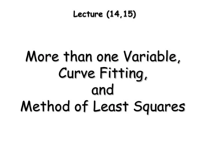
1. Lecture (14,15) More than one Variable, Curve Fitting, and Method of Least Squares

2. Two Variables Often two variables are in some way connected. Observation of the pairs: X Y X1 Y1 X2 Y2 . . . . . . Xn Yn

3. Covariance The covariance gives the some information about the extent to which the two random variables influence each other.

4. x ( )( ) - - y - - x x y y x x y y i i i i 0 3 - 3 0 0 2 2 - 1 - 1 1 3 4 0 1 0 4 0 1 - 3 - 3 6 6 3 3 9 å = = 7 y 3 = x 3 Example Covariance What does this number tell us?

5. Pearson’s R • Covariance does not really tell us anything • Solution: standardise this measure • Pearson’s R: standardise by adding std to equation:

6. Correlation Coefficient

7. Correlation Coefficient (Cont.)

8. Procedure of Best Fitting (Step 1) How to find out the relation between the two variables? 1. Make observation of the pairs: X Y X1 Y1 X2 Y2 . . . . . . Xn Yn

9. Procedure of Best Fitting (Step 2) 2. Make plot of the observations. It is always difficult to decide whether a curved line fits nicely to a set of data. Straight lines are preferable. We change the scale to obtain straight lines.

10. Method of Least Square (Step 3) 3. Specify a straight line relation. Y=a+bX We need to find a and b that minimises the square of the differences between the line and the observed data.

11. = , predicted value = , true value ε = residual error ε Step 3 (cont.)  find best fit of a line in a cloud of observations: Principle of least squares y = ax + b

12. Method of Least Square (Step 4)

13. Method of Least Square (Step 5)

14. Method of Least Square (Step 6)

15. Method of Least Square (Step 7)

16. Example We have the following eight pairs of observations:

17. Example (Cont.) Construct the least square line:  N=8 1/n

18. Example (Cont.)

19. Example (Cont.) Equation Y = 0.545+ 0.636 * X Number of data points used = 8 Average X = 7 Average Y = 5

20. Example (2)

21. Example (3)

22. Excel Application • See Excel

23. Covariance and the Correlation Coefficient • Use COVAR to calculate the covariance Cell =COVAR(array1, array2) • Average of products of deviations for each data point pair • Depends on units of measurement • Use CORREL to return the correlation coefficient Cell =CORREL(array1, array2) • Returns value between -1 and +1 • Also available in Analysis ToolPak

24. Analysis ToolPak • Descriptive Statistics • Correlation • Linear Regression • t-Tests • z-Tests • ANOVA • Covariance

25. Mean, Median, Mode Standard Error Standard Deviation Sample Variance Kurtosis Skewness Confidence Level for Mean Range Minimum Maximum Sum Count kth Largest kth Smallest Descriptive Statistics

26. Correlation and Regression • Correlation is a measure of the strength of linear association between two variables • Values between -1 and +1 • Values close to -1 indicate strong negative relationship • Values close to +1 indicate strong positive relationship • Values close to 0 indicate weak relationship • Linear Regression is the process of finding a line of best fit through a series of data points • Can also use the SLOPE, INTERCEPT, CORREL and RSQ functions

27. Linear Quadratic Cubic General Polynomial Regression • Minimize the residual between the data points and the curve -- least-squares regression Must find values of a0 , a1, a2, … am

28. Polynomial Regression • Residual • Sum of squared residuals • Minimize by taking derivatives

29. Polynomial Regression • Normal Equations

30. Example

31. Example

32. Example Regression Equation y = - 0.359 + 2.305x - 0.353x2 + 0.012x3

33. Nonlinear Relationships To make it linear, take logarithm of both sides • If relationship is an exponential function Now it’s a linear relation between ln(y) and x • If relationship is a power function To make linear, take logarithm of both sides Now it’s a linear relation between ln(y) and ln(x)

34. Examples • Quadratic curve • Flow rating curve: • q = measured discharge, • H = stage (height) of water behind outlet • Power curve • Sediment transport: • c = concentration of suspended sediment • q = river discharge • Carbon adsorption: • q = mass of pollutant sorbed per unit mass of carbon, • C = concentration of pollutant in solution

35. x vs y X=Log(x) vs Y=log(y) Example – Log-Log

36. Example – Log-Log Using the X’s and Y’s, not the original x’s and y’s

37. Example – Carbon Adsorption q = pollutant mass sorbed per carbon mass C = concentration of pollutant in solution, K = coefficient n = measure of the energy of the reaction

38. Example – Carbon Adsorption Linear axes: K = 74.702, and n = 0.2289

39. Example – Carbon Adsorption Logarithmic axes: logK = 1.8733, K = 101.6733 = 74.696, n = 0.2289

40. e x é ù é ù x é ù y x 1n 12 b1 1 1 11 é ù ê ú ê ú ê ú = + e x x b2 y x ê ú ê ú ê ú ê ú 22 2n 2 21 2 ë û bn ê ú ê ú ê ú e x y x x ë û ë û ë û m1 m m m2 mn Multiple Regression • Y1 = x11b1 +x12b2 +…+ x1nbn + e1 Y2 = x21b1 +x22b2 +…+ x2nbn + e2 : Ym = xm1b1 +xm2b2 +…+ xmnbn+ em . Regression model Multiple regression model In matrix notation

41. e x é ù é ù x é ù y x 1n 12 b1 1 1 11 é ù ê ú ê ú ê ú = + e x x b2 y x ê ú ê ú ê ú ê ú 22 2n 2 21 2 ë û bn ê ú ê ú ê ú e x y x x ë û ë û ë û m1 m m m2 mn Multiple Regression (cont.) Observed data = design matrix * parameters + residuals