A Primal-Dual Approach to Online Optimization Problems
730 likes | 1.04k Vues
A Primal-Dual Approach to Online Optimization Problems. Seffi Naor Computer Science Dept. Technion, Haifa, Israel. Based on joint papers with Nikhil Bansal , Niv Buchbinder , and Kamal Jain. TexPoint fonts used in EMF. Read the TexPoint manual before you delete this box.: A A A A A.

A Primal-Dual Approach to Online Optimization Problems
E N D
Presentation Transcript
A Primal-Dual Approach to Online Optimization Problems Seffi Naor Computer Science Dept. Technion, Haifa, Israel Based on joint paperswith Nikhil Bansal, NivBuchbinder, and Kamal Jain TexPoint fonts used in EMF. Read the TexPoint manual before you delete this box.: AAAAA
Road Map Introducing the framework: • Ski rental • Online set cover • Virtual circuit routing The general framework: • General covering/packing linear programs More applications: • The ad-auctions problem • Weighted caching Further research
What is an Online Algorithm? • Input is given “in pieces” over time, each piece is called a “request” • Request sequence: ¾ = ¾1, … , ¾n • Upon arrival of request ¾i : • Online algorithm has to serve the request • Previous decisions for requests ¾1, …, ¾i-1 cannot be changed
Performance Evaluation: Competitive Factor • How to evaluate performance of online algorithm A? • For every request sequence ¾ = ¾1, … , ¾n: • compare cost of A to the cost of an optimal offline algorithm which is given the request sequence in advance • Competitive factor of online algorithm A is ® if • for every request sequence ¾ = ¾1, … , ¾n:
Linear Programming Linear constraints, linear objective Min x1 – 3 x2 + 2 x3 x1 – x2 + 7 x3 <= 2 x2 - x3 >= 0 x1 + 3 x2 + x3 >= -3 Polynomial time solvable. Lies at the heart of optimization.
The Ski Rental Problem • Buying costs $B. • Renting costs $1 per day. Problem: • Number of ski days is not known in advance. Goal: Minimize the total cost.
Ski Rental – Integer Program Subject to: For each day i:
Ski Rental – Relaxation D: Dual Packing For each day i: P: Primal Covering For each day i: • Online setting: • Primal: New constraints arrive one by one. • Requirement: Upon arrival, constraints should be satisfied. • Monotonicity: Variables can only be increased.
Ski Rental – Algorithm D: Dual Packing For each day i: P: Primal Covering For each day i: • Initially x 0 • Each new day (new constraint): • if x<1: • zi 1-x • x x(1+ 1/B) + 1/(c*B) - ‘c’ later. • yi 1
Analysis of Online Algorithm Proof of competitive factor: • Primal solution is feasible. • In each iteration, ΔP ≤ (1+ 1/c)ΔD. • Dual is feasible. Conclusion: Algorithm is (1+ 1/c)-competitive 1-2-3 • Initially x 0 • Each new day (new constraint): • if x<1: • zi 1-x • x x(1+ 1/B) + 1/(c*B) - ‘c’ later. • yi 1
Analysis of Online Algorithm • Primal solution is feasible. If x ≥1 the solution is feasible. Otherwise set: zi 1-x. • In each iteration, ΔP ≤ (1+ 1/c)ΔD: If x≥1, ΔP =ΔD=0 Otherwise: • Change in dual: 1 • Change in primal: BΔx + zi = x+ 1/c+ 1-x = 1+1/c Algorithm: When new constraint arrives, if x<1: zi1-x x x(1+ 1/B) + 1/c*B yi1
Analysis of Online Algorithm • Dual is feasible: Need to prove: We prove that after B days x≥1 x is a sum of geometric sequence a1 = 1/(cB), q = 1+1/B Algorithm: When new constraint arrives, if x<1: zi1-x x x(1+ 1/B) + 1/c*B yi1
Randomized Algorithm 0 1 • Choose d uniformly in [0,1] • Buy on the day corresponding to the “bin” d falls in • Rent up to that day Analysis: • Probability of buying on the i-th day is xi • Probability of renting on the i-th day is at most zi X: X1 X2 X3 X4
Going Beyond the Ski Problem • Ski problem: coefficients in the constraint matrix belong to {0,1} • What can be said about general constraint matrices with coefficients from {0,1}?
The Online Set-Cover Problem • Elements: e1, e2, …, en • Set system: s1, s2, … sm • Costs: c(s1), c(s2), … c(sm) Online Setting: • Elements arrive one by one. • Upon arrival elements need to be covered. • Sets that are chosen cannot be “unchosen”. Goal: Minimize the cost of the chosen sets.
Online Set-Cover: Lower Bound • elements: 1, … ,n • sets: all (n choose n)subsets of cardinality n • cost: unit cost Adversary’s strategy: • While possible: pick an element that is not covered (# of elements offered ≥ n) Competitive ratio: n (cost of online: = n, cost of OPT = 1) But, … n ≈ log(n choose n). polylog(m,n) is not ruled out!
Set Cover – Linear Program D: Dual Packing P: Primal Covering • Online setting: • Primal: constraints arrive one by one. • Requirement: each constraint is satisfied. • Monotonicity: variables can only be increased.
Set Cover – Algorithm D: Dual Packing P: Primal Covering • Initially x(s) 0 • When new element arrives, while • y(e) y(e)+1 • .
Analysis of Online Algorithm Proof of competitive factor: • Primal solution is feasible. • In each iteration, ΔP ≤ 2ΔD. • Dual is (almost) feasible. Conclusion: We will see later. 1-2-3 • Initially x(S) 0 • When new element e arrives, while • y(e) y(e)+1 • .
Analysis of Online Algorithm • Primal solution is feasible. We increase the primal variables until the constraint is feasible. • Initially x(S) 0 • When new element e arrives, while • y(e) y(e)+1 • .
Analysis of Online Algorithm • In each iteration, ΔP ≤ 2ΔD. In each iteration: • ΔD = 1 • Initially x(S) 0 • When new element e arrives, while • y(e) y(e)+1 • .
Analysis of Online Algorithm • Dual is (almost) feasible: • We prove that: • If y(e) increases, then x(s) increases (for e in S). • x(s) is a sum of a geometric series: a1 = 1/[mc(s)], q = (1+ 1/c(s)) • Initially x(S) 0 • When new element e arrives, while • y(e) y(e)+1 • .
Analysis of Online Algorithm • After c(s)O(log m) rounds: We never increase a variable x(s)>1! • Initially x(S) 0 • When new element e arrives, while • y(e) y(e)+1 • .
Conclusion • The dual is feasible with cost 1/O(log m) of the primal. • The algorithm produces a fractional set cover that is O(log m)-competitive. • Remark: No online algorithm can perform better in general. What about an integral solution? • Round fractional solution. (With O(log n) amplification.) • Can be done deterministically online [AAABN03]. • Competitive ratio is O(log m log n).
Online Virtual Circuit Routing Network graph G=(V, E) capacity function u: E Z+ Requests: ri = (si, ti) • Problem: Connect si to ti by a path, or reject the request. • Reserve one unit of bandwidth along the path. • No re-routing is allowed. • Load: ratio between reserved edge bandwidth and edge capacity. • Goal: Maximize the total throughput.
Routing – Linear Program = Amount of bandwidth allocated for ri on path p s.t: For each ri: For each edge e: - Available paths to serve request ri
Routing – Linear Program D: Dual Packing P: Primal Covering • Online setting: • Dual: new columns arrive one by one. • Requirement: each dual constraint is satisfied. • Monotonicity: variables can only be increased.
Routing – Algorithm D: Dual Packing P: Primal Covering • Initially x(e) 0 • When new request arrives, if • z(ri) 1 • . • y(ri,p) 1
Analysis of Online Algorithm Proof of competitive factor: • Primal solution is feasible. • In each iteration, ΔP ≤ 3ΔD. • Dual is (almost) feasible. Conclusion: We will see later. 1-2-3 • Initially x(e) 0 • When new request arrives, if • z(ri) 1 • . • y(ri,p) 1
Analysis of Online Algorithm • Primal solution is feasible. If the solution is feasible. Otherwise: we update z(ri) 1 • Initially x(e) 0 • When new request arrives, if • z(ri) 1 • . • y(ri,p) 1
Analysis of Online Algorithm • In each iteration: ΔP ≤ 3ΔD. If ΔP = ΔD=0 Otherwise: ΔD=1 • Initially x(e) 0 • When new request arrives, if • z(ri) 1 • . • y(ri,p) 1
Analysis of Online Algorithm • Dual is (almost) feasible. We prove: • For each e, after routing u(e)O(log n) on e, x(e)≥1 x(e) is a sum of a geometric sequence x(e)1 = 1/(nu(e)), q = 1+1/u(e) • After u(e)O(log n) requests:
Covering/Packing Linear Programs Primal solutions D: Dual Packing P: Primal Covering P* = D* Dual solutions • ci, aij, bj and the variables xi are all non-negative • Many approximation/exact algorithms are actually primal-dual: shortest path, matching, flows, cuts ..
Key Idea for Online Primal-Dual Primal: Min i ci xi Dual: Max t bt yt Step t, newconstraint:New variable yt a1x1 + a2x2 + … + ajxj≥ bt + bt yt in dual objective xi (1+ ai/ci) xi(mult. update)yt yt + 1 (additive update) primal cost = = Dual Cost
Online Primal-Dual Approach • Can the offline problem be cast as a linear covering/packing program? • Can the online process be described as: • New rows appearing in a covering LP? • New columns appearing in a packing LP? Yes ?? • Upon arrival of a new request: • Update primal variables in a multiplicative way. • Update dual variables in an additive way.
Online Primal Dual Approach Next Prove: • Primal solution is feasible (or nearly feasible). • In each round, ΔP ≤ c ΔD. • Dual is feasible (or nearly feasible). Got a fractional solution, but need an integral solution ?? • Randomized rounding techniques might work. • Sometimes, even derandomization (e.g., method of conditional probabilities) can be applied online! 1-2-3
Simple Lower Bound min x1 + x2 + … + xn x1 + x2 + x3 + … + xn ≥ 1 x2 + x3 + … + xn ≥ 1 x3 + … + xn ≥ ¸1 … xn ≥ ¸1 Online = ¸H(n) ≈ lnn (1+1/2+ 1/3+ … + 1/n) Opt = 1 ( xn=1 suffices) Set all xi to 1/n Increase x2 ,x3,…,xn to 1/n-1 … Increase xn to 1
General Covering/Packing Results {0,1} covering/packing matrix: [Buchbinder Naor 05] • Competitive ratio O(log D) (D: max number of non-zero entries in a constraint). Remarks: • Fractional solutions randomized algorithm (online rounding). • Number of constraints/variables can be exponential. • Possible tradeoff: Competitive ratio/violation of constraints.
General Covering/Packing Results For a general covering/packing matrix [BN05] : Covering: • Competitive ratio O(log n) (n – number of variables). Packing: • Competitive ratio O(log n + log [a(max)/a(min)]) a(max), a(min) – max/min non-zero entry Remarks: • Results are tight. • Can add “box” constraints to covering LP (e.g. x≤1)
Online Primal-Dual Approach Advantages: • Generic ideas and algorithms applicable to many online problems. • Linear Program helps detecting the difficulties of the online problem. • General recipe for the design and analysis of online algorithms. • No potential function appearing “out of nowhere”. • Competitiveness with respect to a fractional optimal solution.
Known Results via P-D Approach Covering Online Problems (Minimization): • O(log k)-algorithm for weighted caching [BBN07] • Ski rental, Dynamic TCP Acknowledgement • Parking Permit Problem [Meyerson 05] • Online Set Cover [AAABN03] • Online Graph Covering Problems [AAABN04]: • Non-metric facility location • Generalized connectivity: pairs arrive online • Group Steiner: groups arrive online • Online multi-cut: (s,t)--pairs arrive online
Known Results via P-D Approach Packing Online Problems (maximization): • Online Routing/Load Balancing Problems [AAP93, AAPFW93, BN06]. • General Packing/routing e.g. Multicast trees. • Online Matching [KVV91]–Nodes arrive one-by-one. • Ad-Auctions Problem [MSVV05]– In a bit …
What are Ad-Auctions? Vacation Eilat You type in a search engine: You get: And … Advertisements Algorithmic Search results
How do search engines sell ads? • Each advertiser: • Sets a daily budget • Provides bids on interesting keywords • Search Engine (on each keyword): • Selects ads • Advertiser pays bid if user clicks on ad. Goal (of Search engine): Maximize revenue
Mathematical Model • Buyer i: • Has a daily budget B(i) • Online Setting: • Items (keywords) arrive one-by-one. • Each buyer gives a bid on each of the items (can be zero) • Algorithm: • Assigns each item to some interested buyer. Assumption: Bids are small compared to the daily budget.
Results [MSVV FOCS 05]: • (1-1/e)-competitive online algorithm. • Bound is tight. • Analysis uses tradeoff revealing family of LP’s -not very intuitive. Our Results [Buchbinder, Jain, N, 2007]: • A different approach based on the primal-dual method. • Techniques are also applicable to further extensions of the problem.
Ad-Auctions – Linear Program I - Set of buyers. J - Set of items. B(i) – Budget of buyer i b(i,j) – bid of buyer i on item j s.t: For each item j: For each buyer i: = 1 j-th ad-auction is sold to buyer i. Each item is sold once. Buyers do not exceed their budget
Ad-auctions Primal and Dual P: Primal Covering For each item j: For each buyer i: For each item j and buyer i: D: Dual Packing
The Primal-Dual Algorithm • Initially: for each buyer i: x(i) 0 • When new item j arrives: • Assign the item to the buyer i that maximizes: • if x(i)≥1 do nothing, otherwise: • - ‘c’ later.
The Paging/Caching Problem Universe of of n pages Cache of size k ¿ n Request sequence of pages: 1, 6, 4, 1, 4, 7, 6, 1, 3, … If requested page is in cache: no penalty. Else, cache miss! load requested page into cache, evicting some other page. Goal: minimize number of cache misses. Question:which page to evict in case of a cache miss?
