Relational Model
Relational Model. Outline. Structure of Relational Databases Relational Algebra - Core Extended Relational Algebra Operations Modification of the Database Views. What is a relation?.

Relational Model
E N D
Presentation Transcript
Outline • Structure of Relational Databases • Relational Algebra - Core • Extended Relational Algebra Operations • Modification of the Database • Views
What is a relation? • Formally, given sets D1, D2, …. Dn a relation r is a subset of D1 x D2 x … x DnThus a relation is a set of n-tuples (a1, a2, …, an) where each ai Di • Example: if customer-name = {Jones, Smith, Curry, Lindsay}customer-street = {Main, North, Park}customer-city = {Harrison, Rye, Pittsfield}Then r = { (Jones, Main, Harrison), (Smith, North, Rye), (Curry, North, Rye), (Lindsay, Park, Pittsfield)} is a relation over customer-name x customer-street x customer-city
Attribute Types • Each attribute of a relation has a name • The set of allowed values for each attribute is called the domain of the attribute • Attribute values are (normally) required to be atomic, that is, indivisible • E.g. multivalued attribute values are not atomic • E.g. composite attribute values are not atomic • The special value null is a member of every domain • The null value causes complications in the definition of many operations • we shall ignore the effect of null values in our main discussion and consider their effect later
Relation Schema • A1, A2, …, Anare attributes • R = (A1, A2, …, An ) is a relation schema E.g. Customer-schema = (customer-name, customer-street, customer-city) • r(R) is a relation on the relation schema R E.g. customer (Customer-schema)
Relation Instance • A relation instance of a relation r corresponds to a table T • An element t of r is a tuple, and corresponds to a row in table T • There is no implied order among the tuples attributes (or columns) customer-name customer-street customer-city Jones Smith Curry Lindsay Main North North Park Harrison Rye Rye Pittsfield tuples (or rows) customer
Database • A database is a collection of relations • Information about an enterprise is broken up into parts, with each relation storing one part of the information E.g.: account : stores information about accountsdepositor : stores information about which customer owns which account customer : stores information about customers • Storing all information as a single relation such as bank(account-number, balance, customer-name, ..)results in • repetition of information (e.g. two customers own an account) • the need for null values (e.g. represent a customer without an account) • Normalization theory deals with how to design relational schemas
Keys • Let K R • K is a superkeyof R if values for K are sufficient to identify a unique tuple of each possible relation r(R) • by “possible r” we mean a relation r that could exist in the enterprise we are modeling. • Example: {customer-name, customer-street} and {customer-name} are both superkeys of Customer, if no two customers can possibly have the same name. • K is a candidate key if K is minimal • Example: {customer-name} is a candidate key for Customer, since it is a superkey (assuming no two customers can possibly have the same name), and no subset of it is a superkey.
Determining Keys from E-R Models • Strong entity set. • The primary key of the entity set becomes the primary key of the relation. • Weak entity set. • The primary key of the relation consists of the union of the primary key of the strong entity set and the discriminator of the weak entity set. • Relationship set. • The union of the primary keys of the related entity sets becomes a super key of the relation. • For binary many-to-one relationship sets, the primary key of the “many” entity set becomes the relation’s primary key. • For one-to-one relationship sets, the relation’s primary key can be that of either entity set. • For many-to-many relationship sets, the union of the primary keys becomes the relation’s primary key
Relational Algebra • A procedural query language based on the mathematical theory of sets that is the foundation of commercial DBMS query languages • Six basic operators • select • project • union • set difference • Cartesian product • rename • The operators take two or more relations as inputs and give a new relation as a result. • Can build expressions using multiple Relational algebra operations
A B C D 1 5 12 23 7 7 3 10 r A B C D A=B D > 5(r) 1 23 7 10 Select Operation p(r) = {t | t rand p(t)} where p is the selection predicate, a formula in propositional calculus consisting of terms connected by (and), (or), (not)Each term is one of: <attribute>op<attribute> or <constant>, where op is one of: = > <
A B C 10 20 30 40 1 1 1 2 r A C A C A,C (r) 1 1 1 2 1 1 2 = Project Operation • A1, A2, …, Ak (r) where A1, A2 are attribute names and r is a relation name. • The result is defined as the relation of k columns obtained by dropping the columns that are not listed in the project list • Duplicate rows removed from result, since relations are sets
A B A B 1 2 1 2 3 = s r r s A B 1 2 1 3 Union Operation • r s = {t | t r or t s} • For r s to be valid, these relations have to be union compatible. 1. r,s must have the same arity (same number of attributes) 2. the domains of the corresponding attributes must be compatible
A B A B 1 2 1 2 3 s r A B = - 1 1 r – s Set Difference Operation r – s = {t | t rand t s} • Set difference must be taken between union compatible relations.
A B C D E 1 2 10 10 20 10 a a b b r s A B C D E 1 1 1 1 2 2 2 2 10 10 20 10 10 10 20 10 a a b b a a b b = x r xs Cartesian-Product Operation r x s = {t q | t r and q s} • Assume that attributes of r(R) and s(S) are disjoint. (That is, R S = ). • If attributes of r(R) and s(S) are not disjoint, then renaming must be used.
Rename Operation • x (E) returns the expression E under the name X If a relational-algebra expression E has arity n, then x(A1, A2, …, An)(E) returns the result of expression E under the name X, and with the attributes renamed to A1, A2, …., An. • Allows us to name, and therefore to refer to, the results of relational-algebra expressions. • Allows us to refer to a relation by more than one name.
Formal Definition • A basic expression in the relational algebra consists of either one of the following: • A relation in the database • A constant relation • If E1 and E2 are relational-algebra expressions then all the following are also relational-algebra expressions • E1 E2 • E1 - E2 • E1 x E2 • p (E1), P is a predicate on attributes in E1 • s(E1), S is a list consisting of some of the attributes in E1 • x(E1), x is the new name for the result of E1
Additional Operations • We define additional operations that do not add any expressive power to the relational algebra, but that simplify common queries. • Set intersection • Natural join • Division • Assignment
A B A B 1 2 1 2 3 r s A B 2 = r s Set-Intersection Operation • rs ={ t | trandts } provided that r, s are union compatible relations • Note that rs = r - (r - s)
r s r s Natural-Join Operation Given two relations r(R) and s(S) their natural join is a relation on schema R S obtained as follows: • for each pair of tuples tr from r and ts from s. • If tr and ts have the same value on each of the attributes in RS then • add a tuple t to the result, where • t has the same value as tr on r • t has the same value as ts on s • Example • if R = (ABCD) and S = (BDE) then • is equal tor.A, r.B, r.C, r.D, s.E (r.B = s.B r.D = s.D (r x s))
B D E A B C D 1 3 1 2 3 a a a b b 1 2 4 1 2 a a b a b = s A B C D E r 1 1 1 1 2 a a a a b r s Natural Join Operation – Example
Division Operation • Given relations r(R=A1…Am, B1…Bn) and s(S=B1…Bn), the the quotient r s is a relation on schema R – S = (A1…Am) defined as r s = { t | t R-S(r) u s ( tu r ) } • Quotients are suited to queries that include the phrase “for all” • It can be shown that r s = R-S (r) –R-S ( (R-S(r) x s) – R-S,S(r)) • Property • If q = r s then q is the largest relation satisfying q x s r • Similar to integer division
A B B 1 2 3 1 1 1 3 4 6 1 2 1 2 = s r s A r Division Example
A B C D E D E a a a a a a a a a a b a b a b b 1 1 1 1 3 1 1 1 a b 1 1 s = r A B C r s a a Division Example
Assignment Operation • The assignment operation () provides a convenient way to express complex queries. • Write query as a sequential program consisting of • a series of assignments • followed by an expression whose value is displayed as a result of the query. • Assignment must always be made to a temporary relation variable. • Example: temp1 R-S (r)temp2 R-S ((temp1 x s) – R-S,S(r))result temp1 – temp2 result
Banking Example Schema branch (branchName, branchCity, assets) customer (customerName, customerStreet, customerOnly) account (accountNumber, branchName, balance) loan (loanNumber, branchName, amount) depositor (customerName, accountNumber) borrower (customerName, loanNumber)
Example Queries • Find all loans of over $1200 • Find the loan number for each loan of an amount greater than $1200 • Find the names of all customers who have a loan, an account, or both, from the bank amount> 1200 (loan) loanNumber (amount> 1200 (loan)) customerName (borrower) customerName (depositor)
Example Queries • Find the names of all customers who have a loan at the Perryridge branch. customerName (branchName=“Perryridge”( borrower.loanNumber = loan.loanNumber(borrower x loan) )) • Find the names of all customers who have a loan at the Perryridge branch but do not have an account at any branch of the bank. customerName (branchName = “Perryridge”( borrower.loanNumber = loan.loanNumber(borrower x loan) )) – customerName(depositor)
Example Queries • Find the names of all customers who have a loan at the Perryridge branch. Query 1customerName(branchName = “Perryridge” ( borrower.loanNumber = loan.loanNumber(borrower x loan) )) Query 2 customerName(loan.loanNumber = borrower.loanNumber( (branchName = “Perryridge”(loan)) x borrower ))
Example Queries • Find the names of all customers who have a loan and an account at bank • Find the largest account balance customerName (borrower) customerName (depositor) balance(account) - account.balance (account.balance < d.balance(account x d (account)))
Query 1 CN(BN=“Downtown”(depositoraccount)) CN(BN=“Uptown”(depositoraccount)) where CN denotes customerName and BN denotes branchName. Query 2 customerName, branchName(depositoraccount) temp(branchName) ({(“Downtown”), (“Uptown”)}) Example Queries • Find all customers who have an account at both the “Downtown” and the Uptown” branches.
customerName, branchName(depositoraccount) branchName (branchCity = “Brooklyn” (branch)) Example Queries • Find all customers who have an account at all branches located in Brooklyn city.
Extended Relational Algebra Operations • Generalized Projection • Extends the projection operation by allowing arithmetic expression over attributes and constants to be used in the projection list • Aggregate Functions • Outer Join
Aggregate Functions and Operations • Aggregation function takes a collection of values and returns a single value as a result. avg: average valuemin: minimum valuemax: maximum valuesum: sum of valuescount: number of values • Aggregate operation in relational algebra G1, G2, …, GngF1( A1), F2( A2),…, Fn( An)(E) • E is any relational-algebra expression • G1, G2 …, Gn is a list of attributes on which to group (can be empty) • Each Fiis an aggregate function • Each Aiis an attribute name • Result of aggregation does not have a name • Can use rename operation to give it a name • For convenience, we permit renaming as part of aggregate operation
branch-name account-number balance Perryridge Perryridge Brighton Brighton Redwood A-102 A-201 A-217 A-215 A-222 400 900 750 750 700 account branch-name balance Perryridge Brighton Redwood 1300 1500 700 branchNameg sum(balance) as total(account) Aggregate Operation Example
Outer Join • An extension of the join operation that avoids loss of information. • First, computes the natural join and then • adds tuples form one of the operand relations that do not match tuples in the other operand relation to the result of the above join • Uses null values: • null signifies that the value is unknown or does not exist • All comparisons involving null are (roughly speaking) false by definition. • Will study precise meaning of comparisons with nulls later
branch-name loan-number amount Downtown Redwood Perryridge L-170 L-230 L-260 3000 4000 1700 customer-name loan-number Jones Smith Hayes L-170 L-230 L-155 Outer Join – Example • Relation loan • Relation borrower
loan-number branch-name amount customer-name L-170 L-230 Downtown Redwood 3000 4000 Jones Smith loan-number branch-name amount customer-name L-170 L-230 L-260 Downtown Redwood Perryridge 3000 4000 1700 Jones Smith null • Left Outer Join: loan Borrower Outer Join – Example • Inner Join: loan Borrower
loan-number branch-name amount customer-name L-170 L-230 L-155 Downtown Redwood null 3000 4000 null Jones Smith Hayes loan-number branch-name amount customer-name L-170 L-230 L-260 L-155 Downtown Redwood Perryridge null 3000 4000 1700 null Jones Smith null Hayes Outer Join – Example • Right Outer Join : loanborrower • Full Outer Join loan borrower
Null Values • It is possible for tuples to have a null value, denoted by null, for some of their attributes • null signifies an unknown value or that a value does not exist. • The result of any arithmetic expression involving null is null. • Aggregate functions simply ignore null values • For duplicate elimination and grouping, null is treated like any other value, and two nulls are assumed to be the same
Null Values • Comparisons with null values return the special truth value unknown • If false was used instead of unknown, then not (A < 5) would not be equivalent to A >= 5 • Three-valued logic using the truth value unknown: • OR: (unknownortrue) = true, (unknownorfalse) = unknown (unknown or unknown) = unknown • AND: (true and unknown) = unknown, (false and unknown) = false, (unknown and unknown) = unknown • NOT: (not unknown) = unknown • In SQL “P is unknown” evaluates to true if predicate P evaluates to unknown • Result of select predicate is treated as false if it evaluates to unknown
Modification of the Database • The content of the database may be modified using the following operations • Deletions • Insertions • Updates • All these operations are expressed using the assignment operator in appropriate relational expressions • For example, deletion and insertion are expressed by r r – E andr r E respectively, where r is a relation and E is a relational algebra query
Views • In some cases, it is not desirable for all users to see the entire logical model • Any relation that is not part of the conceptual model but is made visible to a user as a “virtual relation” is called a view • To define a view with name v that is equivalent to relational algebra query expression E use the statement create view v as E • View definition does not create an actual new relation by evaluating the query expression • Rather, a view definition causes the saving of an expression; the expression is substituted into queries using the view. • One view may be used in the expression defining another view • Database modifications based on views must be translated to modifications of the actual relations in the database. • Some updates through views are impossible to translate into database relation updates