Micro Review (including externalities)
440 likes | 683 Vues
Micro Review (including externalities). Econ 312 Credit to Emma Hutchinson for putting these notes together. They are useful for any microeconomics course with a 103 pre- req. Review of Microeconomics. Reading for Micro Review Your principles of micro text and/or notes O’Sullivan appendix

Micro Review (including externalities)
E N D
Presentation Transcript
Micro Review (including externalities) Econ 312 Credit to Emma Hutchinson for putting these notes together. They are useful for any microeconomics course with a 103 pre-req
Review of Microeconomics • Reading for Micro Review • Your principles of micro text and/or notes • O’Sullivan appendix • In this course we will analyze market outcomes in urban settings with an interest in policy that will correct market failures when such failures occur • Primary questions throughout: • To what outcomes do markets lead? • Under what circumstances are these outcomes desirable? • If markets outcomes are undesirable, what would be the desirable outcome? What is the correct policy response? Econ 312--Farnham
Review of Microeconomics • Analyzing what happens involves positive analysis • Terms desirable and undesirable imply we are also interested in normative analysis. • Positive analysis involves asking what an outcome will be under certain circumstances: • Ex: in equilibrium, how far will people commute to work? • Normative analysis involves asking questions about what outcomes we would like to see. (what should be) • Ex: what is the right (socially optimal) commuting distance? Is an hour drive too long? Why? • Points to the need for a normative criterion by which to judge outcomes as “good” or “bad”. Econ 312--Farnham
Review of Microeconomics • Normative criterion we use in economics is typically that of economic efficiency. • Important to keep in mind that economic efficiency • has utilitarianism as its philosophical base • says nothing (much) about fairness or equity • is only one of many criteria that we can (should?) use to judge market outcomes. • With these caveats in mind, in this class we will (usually) judge outcomes in terms of whether or not they are economically efficient. • Normative statements like “outcome X should happen” should be read as shorthand for “outcome X should happen if we are using economic efficiency as the sole criterion for decision-making.” Econ 312--Farnham
Review of Microeconomics • Economic efficiency defined: • An outcome is efficient if it maximizes net benefits, where net benefits are equal to total benefits minus total costs. • Tells us that, at its core, the analysis of economic efficiency is simply cost-benefit analysis. • We will be analyzing efficiency in a variety of contexts, such as: • What is the efficient level of provision of a public service? • Ex: what is the efficient level of policing? • Should we undertake a particular project (binary decision-making)? • Ex: should Victoria build a light-rail transit system? • How should we allocate a scarce resource across competing uses? • Ex: how much land on the Saanich Peninsula should be used for residential building vs. agriculture vs. public parks? Econ 312--Farnham
Review of Microeconomics • We will focus on answering questions such as these by using cost-benefit analysis to identify the outcomes that make net benefits as large as possible. • Important point: we need to make sure we have correctly identified and measured all of the costs and benefits associated with a given activity/outcome. • An alternative characterization of efficiency (that we may pick up on at various points throughout the term): • An outcome is efficient if it is impossible to come up with an alternative outcome in which at least one person can be made better off without any one person being made worse off. • Although it may not be immediately obvious, we will see that this characterization of efficiency will be satisfied if net benefits are maximized. Econ 312--Farnham
Review of Microeconomics • In order to answer normative questions such as those posed above, we first need to understand how to answer positive questions. • For instance, we need to understand what market outcomes look like, in order to work out whether they are desirable (efficient). • This means we need to recall some basic ideas we learned in principles of microeconomics. • Specifically, we want to understand: • How consumers decide what goods to buy (demand). • How producers decide what goods to produce (supply). • How markets bring producers and consumers together (equilibrium). • Once we understand this, we can assess whether consumers and producers act in such a way as to achieve an economically efficient outcome. Econ 312--Farnham
Review of Microeconomics • Review of Demand. • Three areas to cover on the demand side: • Interpreting an individual consumer’s demand curve • Measuring consumer well-being using the demand curve • Deriving aggregate demand from individual demand Econ 312--Farnham
Review of Microeconomics: Demand • Interpreting an individual’s demand curve • Recall that a demand curve maps out a relationship between price and quantity. Demand curves usually slope downwards: known as the “law” of demand Price (P) Remember, on the horizontal axis we are measuring units of the good consumed (Q), Demand Curve (D) while on the vertical axis we are measuring the price per unit (P), in some form of currency (dollars, cents etc) Quantity (Q) How to interpret this demand curve? Two interpretations, each of which will be useful, depending on the context. Econ 312--Farnham
Review of Microeconomics: Demand • The first interpretation of the demand curve is probably the most familiar to you: Interpretation 1: the D curve tells us how many units of a good a consumer wishes to buy in total, at a given price per unit for the good. P D For instance, the D curve tells us that if the price per unit is P1, then the consumer would like to buy Q1 units. P1 P2 etc. Q1 Q2 Q We can think of this interpretation as reading the D curve horizontally: that is, if we plug in values for P, we get out values for Q. Econ 312--Farnham
Review of Microeconomics: Demand • The second interpretation of the demand curve may be less familiar to you: Interpretation 2: the height of the D curve at any given point tells us how the consumer values additional units of the good. P D For instance, the D curve tells us that if the consumer currently has Q1 units of the good, then a small increase in quantity would be worth P1 per unit to the consumer. P1 P2 etc. Q1 Q2 Q We can think of this interpretation as reading the D curve vertically: that is, if we plug in values for Q, we get out values for P. We will elaborate on this interpretation by use of an example. Econ 312--Farnham
Review of Microeconomics: Demand Example: Suppose that demand is given by Q = 5 - (1/2)P. From the D function, if P=$10, Q=0 will be demanded. But if P = $8, Q = 1 will be demanded. P($) 10 consumer’smaximum willingness to pay for the first unit is greater than $8, but less than $10. 8 Area of the rectangle ($10) thus gives an upper bound on consumer’s willingness to pay for the first unit. D Q 1 5 So we know that the maximum willingness to pay for the first unit is something less than $10. Can we do better than this? Econ 312--Farnham
Review of Microeconomics: Demand Consumer did not buy the first half unit when it cost $5, but does when it costs $4.50. Now consider smaller changes in P. Say Pfrom $10 to $9 so that Qfrom0 to 0.5. P($) consumer’s maximum willingness to pay for this first half unit is something less than $5. 10 9 Now suppose Pfrom $9 to $8, so that total Qfrom 0.5 to 1. 8 Consumer did not buy the second half unit when it cost $4.50, but does when P falls. D Q 5 1 0.5 consumer’s maximum willingness to pay for this second half unit is something less than $4.50. This tells us that the consumer’s maximum willingness to pay for the first unit is in fact something less than $9.50 (as opposed to $10). Econ 312--Farnham
Review of Microeconomics: Demand For instance we could now lower the price in $0.50 increments, rather than in $1.00 increments. We could consider even smaller changes in prices and quantities. P($) Doing this allows us to see that the consumer’s maximum willingness to pay for the first unit is something less than $9.25. 10 9 8 In the limit, as we consider smaller and smaller price changes, what we are doing here is calculating the area under the demand curve between Q=0 and Q=1. D Q 0.5 1 5 This area tells us the exact maximum willingness to pay by this consumer for the first unit of the good. In this case, the area of that trapezoid is equal to $9. The consumer is willing to pay at most $9 for the first unit. Econ 312--Farnham
Review of Microeconomics: Demand By the same logic, the area under the demand curve as we increase Q from 1 to 2 units tells us the maximum willingness to pay for the second unit. In this case, that area equals $7. P($) Indeed, the area under a D curve between any two quantities tells us the maximum willingness to pay for that additional quantity. 10 8 6 If we consider very small increases in quantity, than the trapezoid representing the willingness to pay has a very small base. Q 1 5 2 In the limit, as we consider tiny tiny increases in Q, the base of the trapezoid goes to zero, and the willingness to pay (per unit) for these tiny tiny increases in Q is just equal to the height of the demand curve. Econ 312--Farnham
Review of Microeconomics: Demand This is the logic behind the second interpretation of the demand curve, that the height at any point tells us how consumers value smallQ. As we have seen, this is equivalent to telling us how much the consumer is willing to pay for smallQ. P($) We can also think about this as telling us how much additional benefit a consumer would get from a smallQ. When we are thinking about the D curve in this way, we will refer to it variously as the: Q Marginal Value (MV) curve Marginal Willingness to Pay (MWP) curve Marginal Benefit (MB) curve Note that these terms are equivalent! Econ 312--Farnham
Review of Microeconomics: Demand 1st interpretation of D curve: tells us Q demanded at a given P. • Measuring consumer well-being using the demand curve. 2nd interpretation of D curve: area under the D curve measures consumer’s willingness to pay for Q1 units. P($) But, how much did consumer actually have to pay for Q1? A Expenditure (price times quantity) given by area P1Q1. P1 consumerwilling to pay more than she has to pay. Difference between willingness to pay and expenditure measures consumer well-being. Q Q1 Definition: consumer surplus (CS) = what a consumer is willing to pay minus what they have to pay. In the diagram above, the CS from buying Q1 units at P1 per unit is equal to the triangle A. Econ 312--Farnham
Topic 1(b): Review of Consumer Theory • Deriving aggregate demand from individual demand Suppose two individuals - A and B - each with D curves drawn below. P P Aggregate D DB DA P1 P2 QB QA QA2 QA1 QB2 QB1 QA2+QB2 QA1+QB1 At P1, A demands Q1A and B demands Q1B. Aggregate demand at P1 therefore equals Q1A + Q1B. At P2, A demands Q2A, B demands Q2B, and agg. D = Q2A+ Q2B. We are horizontally aggregating individual demands to get aggregate demand. Econ 312--Farnham
Topic 1: Introduction and Review • Review of Supply. • Three areas to cover on the supply side: • Interpreting an individual producer’s supply curve • Measuring producer well-being using the supply curve • Deriving aggregate supply from individual supply Econ 312--Farnham
Topic 1: Introduction and Review: Supply • Interpreting a firm’s supply curve • Recall that a supply curve maps out a relationship between price and quantity. Supply curves usually slope upwards: known as the “law” of supply Price (P) NB: Throughout this class we will only be looking at the supply behavior of competitive firms. Supply Curve (S) i.e., firms that take the prices of output and inputs as given. Quantity (Q) How to interpret this supply curve? Like D curve, there are two interpretations of the S curve. Econ 312--Farnham
Topic 1: Introduction and Review: Supply • The first interpretation of the supply curve is (again) probably most familiar: Interpretation 1: S curve tells us how many units of a good a producer wishes to sell in total, at a given price per unit for the good. P S P1 If the price per unit is P1, then the firm would like to sell Q1 units. etc, etc. Q1 Q We can think of this interpretation as reading the S curve horizontally: that is, if we plug in values for P, we get out values for Q. Econ 312--Farnham
Topic 1: Introduction and Review: Supply • The second interpretation of the supply curve should also be (relatively) familiar: Interpretation 2: the height of the S curve at any given point tells us how much additional units of the good cost to produce. i.e., the supply curve is also a Marginal Cost (MC) curve. P S P1 If the firm is currently producing Q1 units of the good, then a small increase in quantity would cost P1 per unit to produce. Q1 Q We can think of this interpretation as reading the S curve vertically: that is, if we plug in values for Q, we get out values for P. Again, useful to work through an example. Econ 312--Farnham
Topic 1: Introduction and Review: Supply • Example: Suppose that supply is given by Q = P - 5. From the S function, if P=$5, Q=0 will be supplied. But if P = $6, Q = 1 will be supplied. P($) firm’s cost of supplying that first unit (the MC of that unit) is somewhere between $5 and $6. S 7 6 $12 Turns out that the exact cost of producing this first unit = area under the S curve between Q=0 and Q=1. 5 $6.50 $5.50 Q 2 1 And area under S curve from Q=1 to Q=2 equals cost of producing 2nd unit. And area under S curve from Q=0 to Q=2 tells us how much the firm’s costs increase going from Q=0 to Q=2. Econ 312--Farnham
Topic 1: Introduction and Review: Supply • Area under S curve up to a given Q actually tells us the Variable Cost (VC) of producing that Q. • Recall that a firm’s Total Costs (TC) have 2 components: • TC = Fixed Costs + Variable Costs • = FC + VC. • By definition, FC don’t change as Q changes, while VC do. • So MC = ΔTC/ΔQ =Δ(FC+VC) /ΔQ =ΔVC /ΔQ. • area under the S curve up to a given Q = MC of 1st unit + MC of 2nd unit + MC of third unit etc. etc. • And adding up MCs is the same as calculating VC. Econ 312--Farnham
Topic 1: Introduction and Review: Supply • Measuring producer well-being using the supply curve. 1st interpretation of S curve: tells us Q supplied at a given P. 2nd interpretation of S curve: area under S curve measures VC of producing Q1 units. P($) If producer sells Q1 units at P1 per unit, then Total Revenue (TR) received = area of rectangle P1Q1. P1 producer receives revenue greater than VC. A Difference between TR and VC provides a measure of producer well-being. Q Q1 Definition: producer surplus (PS) = TR - VC. In the diagram above, the PS from selling Q1 units at P1 per unit is equal to the triangle A. Econ 312--Farnham
Topic 1: Introduction and Review: Supply • Measuring producer well-being using the supply curve. • More common measure of producer well-being is profit (π). • What is the relationship between PS andπ? • Recall: • PS = TR - VC; and • π= TR - TC • π= TR - VC - FC π= PS - FC PS or PS = π+ FC. Econ 312--Farnham
Topic 1: Introduction and Review: Supply • Recall that CS measures the NB to consumers from consuming. • Similarly, we can think about PS as telling us about the NB to producers from producing. • That is, tells us how much better off the firm is by choosing Q>0. • If Q = 0, TR=0 and TC=FC. • π = -FC. • If Q>0, TR>0 and TC=FC+VC. • π= PS - FC. • Tells us that maximizingπis equivalent to maximizing PS. • So even thoughπis the “true” measure of firm well-being, we can use PS instead. πas Q=PS as Q Econ 312--Farnham
Topic 1: Introduction and Review: Supply • Deriving aggregate supply from individual firm supply Suppose two firms - A and B - each with S curves drawn below. P SA Aggregate S SB P1 P2 QB QA QB1 QA2 QA1+QB1 QA1 QB2 QA2+QB2 At P1, A supplies QA1 and B supplies QB1. Aggregate supply at P1 therefore equals QA1 + QB1. At P2, A supplies QA2, B supplies QB2, and agg. S = QA2 + QB2. We are horizontally aggregating individual firm supplies to get aggregate supply. Econ 312--Farnham
Topic 1: Introduction and Review • Final topic in Intro/Review: Equilibrium. • Bringing both sides of the market together. • Definition of equilibrium: • a state of balance or rest; • a state where there is no tendency for change. • In our supply and demand model, an equilibrium is where: • Consumers are choosing the Q that makes them happiest, given P. (Consumers choose Q to set MB=P) • i.e., maximizing CS. • Producers are choosing the Q that makes them happiest, given P. (Producers choose Q to set MC=P) • i.e., maximizing PS. • Prices are such that consumer and producer behavior are consistent. • Usually means supply equals demand. (Qs=Qd) Econ 312--Farnham
Topic 1: Introduction and Review: Equilibrium • Example: take the S and D curves illustrated below At price P1, consumers want to buy Q1 units, producers want to sell Q1 units consumer and producer behavior is consistent. P S A B P1 D If P > P1, S > D and there would be pressure on P to fall. Q Q1 At equilibrium of P1 and Q1, NB to consumers = CS = area A and NB to producers = PS = area B. Agg NB = CS + PS = A + B Note that area A is aggregate CS and area B is aggregate PS. That is, CS is sum of all individual consumers’ CS and PS is sum of all individual producers’ PS. Econ 312--Farnham
Topic 1: Introduction and Review: Equilibrium • One very important thing to note: aggregate NB always the same if Q the same, no matter what happens to P. • Another way of saying this is that aggregate NB function only of total Q, while the distribution of NB depends on P. P Example: here equilibrium would be P1, Q1. But, if government imposes a quota at Q2, new equilibrium would be at P2, Q2 where: CS = A PS = B + C + D S A P2 B P1 C Agg NB = CS + PS = A + B + C + D P3 D D Q Q1 Q2 But now suppose that (instead of quota), government instead says P cannot rise above P3 (“price ceiling”). Equilibrium still Q2 but with different P. Now we have: CS = A + B + C PS = D Agg NB = A + B + C + D Same in total, distribution different. Econ 312--Farnham
Topic 1: Introduction and Review • Summary: • We have seen that (absent quotas, price ceilings etc): • Consumers choose Q such that P = MB • i.e., choose to consume where P cuts D curve. • NB to consumers = CS. • Producers choose Q such that P = MC • i.e. choose to produce where P line cuts S curve. • NB to producers = PS. • Producer and consumer decisions are such that S=D • Aggregate NB = sum of individual NB • Sum of individual NB = CS + PS (if consumers and producers are the the only agents affected by the market). • Note that these are positive questions - describing the way in which markets DO work. • Can also ask corresponding normative questions. Econ 312--Farnham
Topic 1: Introduction and Review • Normative questions of interest are: • What quantity of goods should be produced? • We know that in equilibrium Q is where S=D. • Under what circumstances is this the “right” Q in total (the one that maximizes NB)? • Which firms should produce these goods? • We know that in equilibrium each firm produces until P=MC. • Under what circumstances is the the “right” Q for each firm (the one that minimizes aggregate production costs)? • Which consumers should get to consume these goods? • We know that in equilibrium each consumer chooses Q such that P=MB. • Under what circumstances is the the “right” Q for each consumer (the one that maximizes aggregate benefits from consumption)? Econ 312--Farnham
Topic 1: Introduction and Review • We will focus primarily on question (1). The efficient allocation will occur (in all cases discussed in this course) where MC=MB. • Try to understand the intuition for this: • If MC>MB, this tells us the last little bit produced cost more to produce that it gave to consumers in added benefit. Society would be better off with less of the good (Q should fall). • If MC<MB, this tells us the last little bit produced cost less to produce that it gave to consumers in added benefit. This suggest that increasing output would raise overall well-being in society (Q should rise). • If MC=MB, this tells us the last little bit produced cost exactly the same amount to produce as it gave consumers in added benefit. This tells us this unit made society no better off than it was before (nor any worse off). This is the efficient point. • Note that MC=MB in the equilibrium diagram 4 slides back. In a well-functioning market, MC=MB at equilibrium so that the equilibrium is efficient. However, this does not always have to be the case! • When market failure occurs (due to something like the presence of an externality or due to monopolistic control of an industry), it may not be the case that MC=MB at equilibrium • In such a case, the equilibrium quantity may be different from the efficient quantity. Econ 312--Farnham
Externalities—A Typical Cause of Market Failure in Urban Settings • Externalities occur when some market transaction involves costs and/or benefits that accrue to people outside the transaction • This means consumers and producers aren’t taking all of the relevant costs and benefits into account==>Social MB may not equal Social MC in equilibrium. • In such a case, equilibrium is inefficient • In the ideal case we just examined, the only people affected by market transactions were producers and consumers: all costs and benefits in the market were internalized. So (Social MB)=(Social MC) in equilibrium and, therefore, the equilibrium was efficient. Econ 312--Farnham
Some Urban Externalities • Negative externalities (external costs) • Pollution (noise, light, emissions) • Congestion (traffic, sidewalks, parks, etc.) • Spread of disease (especially where water treatment is poor) • Positive externalities (external benefits) • Knowledge spillovers (arguably huge in cities) • “Energy” one feels from being in a bustling city • When externalities are present, market outcomes will typically be inefficient; if the inefficiency is large, this provides solid justification for government intervention in the market (i.e. policy) • In equilibrium, markets produce too much of goods with negative externalities; policy should discourage production • In equilibrium, markets produce too little of goods with positive externalities; policy should encourage production
Externalities—Some Definitions • We defined private costs and benefits previously—those that occur to producers and consumers • Now consider external costs and benefits: those accruing to people outside a market transaction • e.g. Pollution hurts people--it imposes costs on them • Just as we can show the private marginal cost curve for producers in an industry, we can think of the marginal external cost imposed on others by different levels of production. • If we add up the marginal private costs and marginal external costs of production, we get the overall marginal social cost of production. (mpc+mec=msc) • Marginal social cost curve describes the costs, on the margin, imposed on both producers and people external to the transaction, for different levels of production. Note that mec can be positive (in the case of negative production externalities) or negative (in the case of positive production externalities—like information spillovers between firms)
Externalities—Some Definitions • Similarly marginal social benefits are the marginal private benefits plus marginal external benefits (mpb+meb=msb) • meb can be positive (in the case of positive consumption externalities) or negative (in the case of negative consumption externalities) • We show production externalities using MC curves. • We show consumption externalities using MB curves
MEC is vertical distance between MPC and MSC Equilibrium at Qeqwhere S=D But is this efficient? MSC=MPC+MEC MSC>MSB at Qeq implies that too much is being produced Want MSC=MSB! Qeff is efficient level of production Consider a negative production externality (MEC>0) MSC P S=MPC Peq D=MSB Q Qeq Qeff Econ 312--Farnham
What does society gain from moving from Qeqto Qeff? Loses total social benefits of E Gains total social cost reduction equal to D Net gain of F Note that F is equilibrium deadweight loss Social Welfare (SW) society could have if only it moved from Qeqto Qeff. Neg Production Externality--Welfare Analysis loss= E =gain D MSC P S=MPC F Peq D=MSB Q Qeq Qeff Econ 312--Farnham
Taxes generally reduce SW when equilibrium is efficient (market success) Taxes Can be SW improving for mkt failure w/neg externality, can restore Qeff Impose tax that sets t=MEC at Qeff SW after tax equals areas CS+PS+GR-TEC CS= GR= PS= Policy Example: Using a per unit tax to correct a pollution externality TEC= MSC P S(w/tax) t=MEC(Qeff) Pc S=MPC Peq Ps D=MSB Q Q’eq=Qeff Qeq Econ 312--Farnham
Social welfare in this case is the area shown to the right. It’s CS plus the part of GR not cancelled out by TEC. Note that PS is cancelled out by part of TEC Social Welfare SW With Tax-Corrected Externality SW CS+GR+PS TEC - = Econ 312--Farnham
Suppose a constant MEB results from production activity (knowledge spillovers?); show externality with S curve Vertical shift (down) of S curve by amount of MEB MSC=MPC-MEB MSB=MPB because no externality on consumption side Too little produced in equilibrium Positive production externality Now Consider a Positive Production Externality P S=MPC MSC Peq MEB D=MPB=MSB Q Qeq Qeff Econ 325--Martin Farnham
What is correct policy response? • Work this out on your own • Remember, you want to encourage increased production of this good • Do graphical welfare analysis • Show how a policy instrument can be used to correct the market failure. Econ 312--Farnham