Download
1 / 34
350 likes | 588 Vues
What are firms goals?. The motivation for business decisions is profit maximization. How? Increase revenue. Decrease costs. Compete in the market place. Survive – Stronger . What are firms goals?. Increase revenue. TR = P x Q Decrease costs.

E N D
What are firms goals? • The motivation for business decisions is profit maximization. • How? • Increase revenue. • Decrease costs. • Compete in the market place. • Survive – Stronger
What are firms goals? • Increase revenue. • TR = P x Q • Decrease costs. • Technology, efficiency, productivity, cost cutting, labor vs. capital, domestic vs. foreign, substitution • Profit = TR - TC • Compete in the market place. • Mergers and acquisitions (Standard Oil) , predatory pricing, unfair trading practices, consumers vs. produces (Japan) • Economies of scale, Dumping practices
What is the difference between accounting costs and opportunity costs? To distinguish between the way economists measure costs and the way accountants measure costs
Item Accounting Profit Economic Profit Computech’s Accounting Versus Economic Profit Total Revenue Less Explicit costs: Wages & salariesMaterialsInterest paidOther payments Less implicit costs:Foregone salaryEconomic Dep. Foregone interest Equals profit $500,000 $420,000 $300,000$100,000$10,000$10,000 000 $80,000 $500,000 $420,000 $300,000$100,000$10,000$10,000 $115,00080,00030,000 5,000 -$35,000 Exhibit 1
Item Accounting Profit Economic Profit Computech’s Accounting Versus Economic Profit Total Revenue Less Explicit costs: Wages & salariesMaterialsInterest paidOther payments Less implicit costs:Foregone salaryEconomic DepForegone interest Zero economic profit $535,000 $300,000$100,000$10,000$10,000 000 $115,000 $535,000 $300,000$100,000$10,000$10,000 80,00030,0005,000 $0 Exhibit 1
What are Explicit Costs? • Direct costs • A cost paid in money • Payments to nonowners of a firm for their resources • Accounting costs • Cash payment
Example of Explicit Costs • Wages • Raw materials • Interest rates to the bank and bond holders • Utility • Other direct payments
What are Implicit Costs? • The opportunity cost incurred by a firm when it uses a factor of production for which it does not make a direct money payment. • The opportunity cost of using resources owned by the firm • Indirect costs • Hidden costs • Non-payment costs • Owners costs
Example of Implicit Costs? • Forgone salary • Forgone rent • Forgone interest on investment. • Economic depreciation (change in market value of capital over time)
Accounting profits = • Accounting Profits • Profit = Total revenue – Total Costs • (explicit costs) • Profit = P x Q - TC (FC + VC) • Economic Profits = Total revenue – TC + Opportunity costs (Explicit+Implicit) • Accounting profits are always greater than economic profits
What are Fixed Costs? • Fixed Costs • Sunk Costs • Q = 0 ……….FC ….. + (Positive) • As Q (increases) FC remains the same • Examples • Rent • Insurance; taxes • Interest Payment
Example:Renting a class (Maximum 25 students) • Q=0 …FC = $1000 ….AFC = $1000 • Q=5 …FC = $1000 …. AFC = $200 • Q=10…FC = $1000 ….AFC = $100 • Q=15 …FC = $1000 …AFC = $66 • Q=20 ….FC = $1000…AFC = $50 • Q=25 ….FC = $1000…AFC = $40
What are Variable Costs? • Variable Costs Q = 0 ……….VC ….. 0 (zero) • As Q (increases) VC • Examples • wages • Utility • Raw materials
AFC = TFC/TQ • AVC=TVC/TQ • ATC=TC/TQ=FC+VC/TQ • MC = TC/ Q • MC = cost of producing one additional unit of a product • MC = • (+) or (– ) or ( )
950 640 775 550 525 566.6 425 400 400 350 325 400 306 300 280 300 220
What is the Marginal-Average Rule? When MC < AC, AC falls When MC > AC, AC rises If MC = AC, AC at minimum Grade point average
L TP MP 0 0 1 1 2 3 3 6 4 8 5 9 6 9 A 1 B 2 C D 3 E 2 F 1 0 G H -1 7 8
Total Product 9 9 9 8 8 8 7 6 6 5 Marginal Product 4 3 3 Average Product 2 1 1 1 2 3 4 5 6 7 8 9 B F
Increasing marginal returnsDecreasing marginal returns • Specialization • Division of labor • Learning curve • Same work space • limited equipment • bureaucracy • command and control • specialization but decreasing importance
Shifts in cost curve • Technology • Product curve • Cost curve down • Prices of factors of production • Product curve • Cost curve down
What is Normal Profit? • The minimum profit necessary to keep a firm in operation • Covering all costs • Direct costs (explicit) (FC+VC) • Indirect costs (implicit) opportunity costs • Zero economic profit is good. Why?
Item Accounting Profit Economic Profit Computech’s Accounting Versus Economic Profit Total Revenue Less Explicit costs: Wages & salariesMaterialsInterest paidOther payments Less implicit costs:Foregone salaryEconomic DepForegone interest Zero economic profit $535,000 $300,000$100,000$10,000$10,000 000 $115,000 $535,000 $300,000$100,000$10,000$10,000 80,00030,0005,000 $0 Exhibit 1
Golden rule for profit maximization or loss minimization • Always produce where MC = MR. Why ? • MR = TR/ Q • How is the price determined in the market?
Plant Size and Cost ( Q ) • Economies of scale • specialization, division, learning curve, overhead spread, market power, • Diseconomies of scale • Diseconomies of scale arise from the difficulty of coordinating and controlling a large enterprise. • Eventually, management complexity brings rising average total cost. • Constant returns to scale • Constant returns to scale occur when a firm is able to replicate its existing production facility including its management system.
LONG-RUN COST Figure 11.9 shows a long-run average cost curve. In the long run, Samantha can vary both capital and labor inputs. With its current plant, Sam’s ATC curve is ATC1. With successively larger plants, Sam’s ATC curves would be ATC2,ATC3, and ATC4.
LONG-RUN COST The long-run average cost curve, LRAC, traces the lowest attainable average total cost of producing each output.
LONG-RUN COST Sam’s experiences economies of scale as output increases to 9 gallons an hour, … constant returns to scale for outputs between 9 gallons and 12 gallons an hour, … and diseconomies of scale for outputs that exceed 12 gallons an hour.
The ATM and the Cost of Getting Cash The average total cost curve for transactions with a human teller is ATCT. The lowest average total cost for a human teller transaction is $1.07. The average total cost curve for transactions with an ATM is ATCA. The lowest average total cost curve for an ATM transaction is 27 cents.
The ATM and the Cost of Getting Cash The long-run average cost curve is LRAC. At Q transactions per month, both methods have the same average total cost. For a credit union that does fewer than Q transactions per month, its least-cost method is the teller. For a bank that does more than Q transactions per month, the least-cost method is the ATM.
The ATM and the Cost of Getting Cash More technology and more capital is not always efficient.