Download
1 / 27
270 likes | 485 Vues
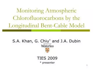
Monitoring Atmospheric Chlorofluorocarbons by the Longitudinal Bent-Cable Model. S.A. Khan, G. Chiu * and J.A. Dubin. TIES 2009 * presenter. Outline. Introduction CFC-11 Data Model Inference Results Further Extension of the Methodology Limitations. Introduction.

E N D
Monitoring Atmospheric Chlorofluorocarbons by the Longitudinal Bent-Cable Model S.A. Khan, G. Chiu* and J.A. Dubin TIES 2009 * presenter
Outline • Introduction • CFC-11 Data • Model • Inference • Results • Further Extension of the Methodology • Limitations
Introduction • Concentration of CFC-11 in response to the Montreal Protocol’s ban on CFC products (monitored from Mauna Loa) Outgoing Phase (0 - 2 ) + (1 + 2) ti Transition period Incoming Phase CTP: the point at which it took a downturn from an increasing trend 0 + 1 ti • Shock-through data – a trend characterized by a change due to a shock (the Montreal Protocol) - + Figure 1: Characterizing a trend of shock-though data by the bent-cable function
Introduction (cont’d) • Bent-cable function (Chiu, Lockhart & Routledge, 2006) f(xi, , ) = 0 + 1 ti + 2 q(ti, ), where = (0 , 1,2), = (, ), q(ti, ) = , • Bent-cable Regression: yi = f(ti, , ) + i • i iid (Chiu, Lockhart & Routledge, 2006, JASA) • i AR(p) (Chiu and Lockhart, revisions submitted) • R Package ‘bentcableAR’ handles both
Introduction (cont’d) • We have extended the bent-cable regression for longitudinal data using random coefficients and within-individual noise that is AR(p), p 0 • We have applied our methodology to CFC-11 data monitored from different stations all over the globe (Khan, Chiu & Dubin, to appear in CHANCE, 2009)
CFC-11 Data Reduction of Ozone Layer in the Upper Atmosphere Natural (followed by a natural recovery) Human Activities (e.g. use of CFCs) Skin Cancer and Cataracts Reduction of Organisms in the Ocean’s Photic Zone Increased UV Exposure Damage to Plants
CFC-11 Data (cont’d) CFCs (11, 12, 113, 114, 115) CFC-11: One of the most dangerous CFCs to reduce the ozone layer in the atmosphere (ODP = 1) Nontoxic, nonflammable chemicals containing atoms of carbon, chlorine and fluorine Used in air conditioning/cooling units, and aerosol propellants prior to the 1980’s Destroy Ozone Banned globally by the 1987 Montreal Protocol
CFC-11 Data (cont’d) Pt. Barrow, Alaska Ragged Point, Barbados Mace Head, Ireland Cape Matatula, American Samoa Niwot Ridge, Colorado Mauna Loa, Hawaii South Pole, Antarctica Cape Grim, Tasmania Monitoring stations of CFCs all over the globe (Data collected by NOAA/ESRL global monitoring division and ALE/GAGE/AGAGE global network program)
CFC-11 Data (cont’d) • What were the rates of change before and after the transition period? • How long did it take to show an obvious decline? • What was the CTP at which the trend went from increasing to decreasing? CFC-11 profiles of eight stations (monthly mean data)
Model • fij = f(tij, i, i), qij =q(tij, i) • i = (0i, 1i, 2i)', i = (i, i)' • = (1, … , p)' • yi(1) = (yi1, …, yip)' • yi(2) = (yi,p+1, …, )' Level 1 • yij = fij + ij, • yij = ij + uij, j = p+1, …, ni • Yij| yi1, …, yip, i, i, , • Yi(2)| yi(1), i, i, , ~ MVN(i, Ii), where, i = (i,p+1, … , )'
Model (cont’d) Level 2 • i and i are independent • i| , D1 ~ MVN(, D1), i| *, D2 ~ BVLN(*, D2) Level 3 • , ~ MVN(h, H) • ~ MVN(h1, H1) , * ~ BVN(h2, H2), • ,
Inference Bayesian inference for longitudinal bent-cable regression Implementation MCMC (Metropolis Within Gibbs) Full conditionals • Drawing MCMC • samples • – C • MCMC output • Analysis • – R (coda package) (1) i|. (2) i|. (3) (4) (5) (6) |. (7) *|. (8) |. Computation
i|. ~ Normal i|. ~ No closed-form expression ~ Gamma ~ Wishart ~ Wishart |. ~ Normal *|. ~ Normal |. ~ Normal Inference (cont’d)
Results assuming AR(1) within-station noise • Black: Observed data • Red: Station-specific fit • Green: Population/ global fit • Estimated transition is marked by the vertical lines
Results (cont’d) • Black: Observed data • Red: Station-specific fit • Green: Population/ global fit • Estimated transition is marked by the vertical lines
Results (cont’d) • Global • Significant increase/decrease in CFC-11 in the incoming/outgoing phases • incoming phase:average increase in CFC-11 was about 0.65 ppt/month during the • outgoing phase: average decrease was about 0.12 ppt/month • Transition: Global drop in CFC-11 took place between Jan ’89 and Sep ’94, approximately • Estimated CTP was Nov ’93 • CFC-11 went from increasing to decreasing in around Nov ’93
Results (cont’d) • Station-Specific • Significant increase/decrease of CFC-11 in the incoming/outgoing phases for all stations individually • Rates at which these changes occurred agree closely • Approximately constant rates of change before and after the enforcement of the Montreal Protocol, observable despite a geographically spread-out detection network
Results (cont’d) • Station-Specific • Transition periods and CTPs varied somewhat across stations • This may be due to the extended phase-out schedules contained in the Montreal Protocol – 1996 for developed countries and 2010 for developing countries • Durations of the transition periods are very similar among stations except for South Pole
Results (cont’d) • Station-Specific (South Pole) • Highly unusual weather conditions • CFCs are not disassociated during the long winter nights • It may be expected for CFCs to remain in the atmosphere for a long period of time, and hence, an extended transition period Outlier CFC-11 measurements showed little variation over time
Results (cont’d) • Key Findings • Substantial decrease in global CFC-11 levels after the gradual transition suggest The Montreal Protocol, which came into force in Jan ’89, can be regarded as a successful international agreement to reduce the atmospheric concentration of CFCs globally • The rate by which CFC-11 has been decreasing suggests that it will remain in the atmosphere throughout the 21st century, should current conditions prevail
Further Extension of the Methodology Gradual change ( > 0) Abrupt change ( = 0)
Further Extension of the Methodology (cont’d) Gradual ( > 0)? Abrupt ( = 0)?
Further Extension of the Methodology (cont’d) Longitudinal bent-cable Methodology for smooth/gradual transition √ What if the sample comes from two potential populations: one with a gradual transition period, and the other with an abrupt transition? Longitudinal bent cable to account for either type of transition – gradual or abrupt – driven by the data rather than assuming that only one type is possible Flexible methodology for longitudinal changepoint data
Limitations • Assumes stationarity of the AR process • Can be sensitive to the values of the hyper-prior parameters • Example: If the AR process is close to non-stationary, a restrictive prior for could be required • in progress: alternative modeling approach and/or prior specification for (e.g. Fisher transformation)