Chapter 4 Color in Image and Video

1. Chapter 4Color in Image and Video 4.1 Color Science 4.2 Color Models in Images 4.3 Color Models in Video 4.4 Further Exploration

2. Chapter 4Color in Image and Video 4.1 Color Science 4.2 Color Models in Images 4.3 Color Models in Video 4.4 Further Exploration

3. Light and Spectra Light is an electromagnetic wave. Its color is characterized by the wavelength content of the light. • Laser light: • consists of a single wavelength: e.g., a ruby laser produces a bright, scarlet-red beam. • Most light sources: • produce contributions over many wavelengths. • Visible wavelengths: • humans cannot detect all light, just contributions that fall in the “visible wavelengths". • From Blue to Red: • Short wavelengths produce a blue sensation, long wavelengths produce a red one.

4. Spectrophotometer device used to measure visible light, by reflecting light from a diffraction grating (a ruled surface) that spreads out the different wavelengths.

5. Daylight (white light) E() • White light contains all the colors of a rainbow. • Visible light is an electromagnetic wave in the range 400 nm to 700 nm • “nm” stands for nanometer (10−9 meters) E(): Spectral Power Distribution (SPD) or spectrum.

6. Human Vision • Lens (水晶體) and Retina (視網膜) • The eye works like a camera. • Lens focus an image onto the retina (upside-down and left-right reversed). • Rods (柱狀體) and Cones (錐狀體) • Rods: “all cats are gray at night!“ • Three kinds of cones: most sensitive to red (R), green (G), and blue (B) light. • Eye-Brain System • The brain is good at algebra.

7. Spectral Sensitivity Curves(1) Spectral Sensitivity Functions qR(), qG() and qB()

8. Spectral Sensitivity Curves (2) Fig 4.3 R, G, B cones, and Luminous Efficiency Curve V()

9. Luminous Efficiency Function • 6 millions of cones • proportion of R:G:B ~ 40:20:1 • Luminous Efficiency Function V () • sum of the response curves for R, G, and B. • The rod sensitivity curve: • looks like the luminous-efficiency function V () but is shifted to the red end of the spectrum.

10. Spectral Sensitivity of the Eye • These spectral sensitivity functions • q () = (qR(), qG(), qB())T(4.1) • The response in each color channel in the eye is proportional to the number of neurons firing. • R = E() qR() d  G = E() qG() d  B = E() qB() d  (4.2)

11. Surface Reflectance S() • Fig. 4.4 surface spectral reflectance • (1)orange sneakers • (2) faded bluejeans. • S():reflectance • function

12. Fig 4.5 Image formation model

13. Color Signal C() • Light from the illuminant with SPD E() impinges on a surface, with surface spectral reflectance function S(), is reflected, and then is filtered by the eye's cone functions q (). • Reflection is shown in Fig. 4.5 below. • The function C() is called the color signaland consists of the product of E(), the illuminant, times S(), the reflectance: C() = E()S().

14. Image formation • The equations that take into account the image formation model are: R = E() S() qR() d  G = E () S() qG() d  B = E() S() qB() d  (4.3)

15. (break)

16. Color-Matching Functions • A technique evolved in psychology • Matching a combination of basic R, G, and B lights to a given shade • (even without knowing the eye-sensitivity curves of Fig.4.3) • Color Primaries • 700, 546,436 – nm (700, 546.1,435.8) • 580, 545,440 – nm  Error / mistake? 課本這段是錯的，Google “CIE 1931”

17. Colorimeter 700 nm 546 nm 436 nm Fig 4.8 Colorimeter experiments

18. CIE 1931 2° Matching Func. 700 nm 546 nm 436 nm Radiant power 72 : 1.3791 : 1 Fig 4.9 CIE RGB color matching functions

19. Recall:Spectral Sensitivity l=560, for example Spectral Sensitivity Functions qR(), qG() and qB()

20. Recall: CIE 1931 2° 700 nm 546 nm 436 nm l=560, for example Fig 4.9 CIE RGB color matching functions

21. Relation Between 2 Exps. [ E(l) ] M 加乘轉換矩陣 (M) 三色光轉換成各別 刺激度再加總 單光源 刺激度 單位能量 配色比 l=436  r(436)=0, g(436)=0, b(436)>0 l=546  r(546)=0, g(546)>0, b(546)=0 l=700 r(700)>0, g(700)=0, b(700)=0

22. [R G B] Stimulus RGB單一色彩的刺激 也是暫定三原色的組合 (紅色的刺激不能只靠暫定紅光模擬)

23. CIE 1964 10° Matching Func. 另取「暫定三原色」亦無法改變紅光的負值 645 nm 526 nm 444 nm Normalized by Radiant power to 1 : 1 : 1

24. Grassman's Law 配色函數無法呈現色光的加法定理 • Additive color • results from self-luminous sources • lights projected on a white screen • phosphors glowing on the monitor glass • Additive color matching is linear. • color1  a linear combinations of lights • color2  another set of weights, then • combined color: color1+color2  the sum of the two sets of weights.

25. Grassman's Law (Example) • Example • color1  0.2 X + 0.6 Y + 1.2 Z • color2  1.8 X + 0.9 Y + 0.3 Z • color1+color2  2 X + 1.5 Y + 1.5 Z • Example 2 (線性內插: 假設色彩有坐標) • color1  (0.2 X + 0.6 Y + 1.2 Z) /2 • color2  (1.8 X + 0.9 Y + 0.3 Z) /3 • (1/2) color1+ (1/2) color2  0.35 X + 0.3 Y + 0.35 Z

26. Drawback of the RGB Color Matching Functions • RGB stimuli are dependent on linear combinations of r(), g() , b() , but not purely respective values of them. • r() color-matching curve has a negative lobe • Thus we cannot conveniently indicate a combined color following Grassman’s law • qR(575)!= qR(550)/2+qR600)/2

27. CIE-RGB to CIT-XYZ Fig 4.10 CIE standard XYZ color matching Functions x(), y(), z(). 下一頁：改用「坐標軸」來看待「調色」

28. Linear Transform (RGB-XYZ) 由「暫定三原色」經線性轉換， 定義出「虛擬三原色」。

29. Fictitious Primaries • A 3 x3 matrix away from r, g, b curves, and are denoted x(), y(), z(), as shown in Fig. 4.10 • XYZ color-matching functions with only positives values • The middle standard color-matching function y() exactly equals the luminous-efficiency curve V () shown in Fig. 4.3. • The area under Each curve is the same.

30. Orthogonal XYZ Color Space • Original Coordinate before Normalization • Pure Colors without Combination

31. CIE Chromaticity Diagram (4.6) (4.10) (4.7) (4.8) z = 1 – x – y (4.9)

32. (x,y) Chromaticities Fig 4.11 Recall: Grassman’s Law Spectrum Locus horseshoe B A C Line of purples

33. Chromaticities and White points of Monitor Specification 4.1.9 Table 4.1

34. Out-of-Gamut Colors 4.1.10 Fig. 4.13: Approximating an out-of-gamut color

35. Additive Color (1) In nature (2) Powerpoint: NA (3) Expert software: [R3 G3 B3] = ( a[R1 G1 B1] + b[R2 G2 B2] )/(a+b)

36. (break)

37. Extra Topics of Additive Color Models • YUV Color Model • YIQ Color Model • YCbCr Color Model • L*a*b* (CIELAB) Color Model • Munsell Color Naming System

38. RGB  YUV • Y= 0.229 R + 0.587 G + 0.114 B • U=B-Y • V=R-Y

39. YUV Decomposition

40. (R+G+B)/3 Y channel

41. YIQ Color Model • YIQ is used in NTSC color TV broadcasting • “Y“ in YIQ is the same as in YUV; • I and Q are a rotated version (33° ) of U and V . I Q

42. YIQ Transform Matrix

43. YCbCr Color Model • ITU Standard (International Telecommunication Unit) • ITU-R BT. 601-4 (also known as “Rec. 601”) • Closely related to the YUV transform

44. YCbCr Transform Matrix Theoretical: Digital Processing: (16~235/ ± 112+128)

45. L*a*b* (CIELAB) Color Model Outside solid More colorful (saturate) Max b* Yellow Min b* Blue Max a* Red Min a* Green Fig 4.14 CIELAB Model

46. Munsell Color Naming System

47. More Color Coordinate Schemes • HSL -- Hue, Saturation and Lightness; • HSV -- Hue, Saturation and Value; • HSI -- Hue, Saturation and Intensity; • HCI -- C=Chroma; • HVC -- V=Value; • HSD -- D=Darkness; • CMY -- Cyan(C), Magenta(M) and Yellow(Y ) color model.

48. Gonzalez. Chapter 6 Color Image Processing

49. Gonzalez.Chapter 6 Color Image Processing

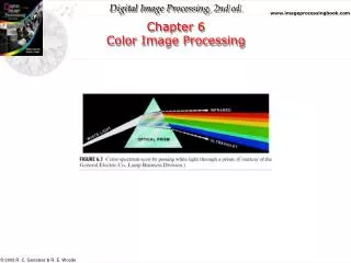
50. Gonzalez.Chapter 6 Color Image Processing