Download

1 / 26
260 likes | 364 Vues
OBER simulation science: direction/needs of the next 2-5 years. Doug Rotman, LLNL Feb. 22, 2001 NERSC-NUGEX meeting February 22/23, 2001. OBER’s simulations will continue to challenge compute platforms of the next decade. Climate modeling and carbon cycle

E N D
OBER simulation science: direction/needs of the next 2-5 years Doug Rotman, LLNL Feb. 22, 2001 NERSC-NUGEX meeting February 22/23, 2001
OBER’s simulations will continue to challenge compute platforms of the next decade • Climate modeling and carbon cycle • Atmospheric chemistry and aerosols • Computational biology
Understanding climate forcings Global, annual-mean radiative forcings (W m-2) due to a number of agents from 1750 to present. The vertical line about the rectangular bar indicates an estimate of the uncertainty range [IPCC, 2000a].
Climate modeling: current capabilities • Coupled atmos/ocean (resolution) • atmos: about 2 degrees • ocean: about 1 degree • Atmos: prescribed land types, substantial efforts in radiation physics (SW/LW), boundary layer physics, cloud physics, and meteorological processes • Ocean: detailed ocean floor topography, convection • includes atmospheric sulfate aerosols • prescribed greenhouse gases - CO2, ... • model top ~ 40-50 Kms • Multi-century simulations are large productions • Ensembles of multi-century are heroic
Climate Modeling parallel computing characteristics • Mostly 1-D domain decomposition • At current resolution, focused on ~100-200 processors • Typically not memory bound • Throughput is major issue • Climate simulations tend to be long, hence queuing system to enable long running jobs is optimal (but, we are also quite talented at playing the queuing games!) • more general 2-D (and 3-D!!) decompositions are coming ...
Moving to higher resolution climate models • Topology, land types, clouds, precipitation, emissions of species, … all point to the need for higher resolution climate simulations to understand processes that impact climate prediction • There are multiple scientific issues to be addressed at higher resolution, but, … • To 1st order, computational limitations dominate
Higher resolution costs build quickly (15 year run in 8 hours wall clock) Resolution (km) Required (Gflops) Required storage (Gbytes) 300 15 25 200 32 50 150 140 120 125 220 190 75 1330 620 60 3300 1450 40 22000 4900 30 42000 7600 Just monthly averages! Grid size Sustained!
Future climate models will include chemistry and more complete aerosol physics • Accurate modeling of atmospheric processes and climate requires inclusion of realistic ozone chemistry and aerosol direct and indirect effects • Chemistry and aerosols provide intense, but local calculations • Transport of chemical species provides communication and accuracy challenges Obs Increasing chemistry and physics
Moving from Specified to Predicted CO2 • We must move from this: Specified Atmospheric CO2 Concentration Climate Model Future Climate • To this: Integrated Climate and Carbon Model CO2 Concentration Specified CO2 Emissions Future Climate
DOCS/LLNL CO2 injection near New York City at 3000 m depth. Shown isthe amount of injected CO2 per unit surface areaafter 100 years of continuous injection. Carbon management requires knowledge of sources, sinks and reservoirs Carbon cycle modeling requires interactive atmospheric, ocean and terrestrial ecosystem models (A) Ocean carbon column inventory and (B) fluxes of anthropogenic carbon as of 1995
Need linkage to terrestrial ecosystem models • How does vegetation and soils change with respect to changes in land use or climate?
Next Generation Internet: Creating a Earth System Grid • Goal: Enable a geographically distributed climate community [of thousands] to perform sophisticated, computationally intensive analyses and visualization on Petabytes of data • Approach: We are integrating advanced data structures and algorithms for analysis and visualization of petabyte data in a distributed environment. • Collaborators: NCAR, LBNL, ANL, LANL
Atmospheric chemistry: Current capabilities NO2 at 30 Km • Separate stratospheric and tropospheric models (almost) • resolution: about 2-4 degrees horizontal and 2 Km vertical • short simulations using more complete mechanisms (80-100 species), multi-year runs use smaller chemistry(30-50 species); still uncertainty on some rates, ... • substantial parameterizations, but still large uncertainties (dry dep, scavenging, PBL diffusion, …) • fixed emissions, need interactive ... • aerosols use fixed size distribution and many times, fixed geographic distribution • little feedback to climate model
We can now simulate ozone in a combined troposphere and stratosphere: will become standard
Chemistry coupling to biogeochemical ocean models • Chlorophyll: provides feedback to DMS and sulfur emissions, which then impacts sulfate aerosol and climate forcing Dec 1996, pre-El Ninos Dec 1997, strong El Ninos
Formation of sulfate aerosols is dependent on local ozone concentration Rather than using monthly averaged ozone distributions, we are now moving forward to calculate aerosol formation using interactive and local ozone Interactive chemistry and aerosols
Aerosol indirect effects may be more important than direct effects • Direct effects of aerosol (scattering) has been included • Indirect effects (brightness and lifetime of clouds) may be more important and needs to be included • microphysics plays a role; models will be implementing algorithms for the evolution of the aerosol size distribution via sedimentation, coagulation, nucleation, …. • Interaction between aerosol microphysics and cloud physics is still very uncertain W/m2
General Computational needs for future climate/chemistry modeling • Hardware • Sustained performance of about 250 Gflops • Peak flop to byte (on processor): 2 to 1 • Aggregate memory: 1-2 Tbytes • Cache at least 8 mb, hopefully 16mb • Inter-node, bi-directional bandwidth: 1 - 5 Gbytes • Latency: 5 micro-seconds • Aggregate I/O bandwidth: 8 Gbytes/sec • Disk needs: 10-50 Tbytes • Software • MPI and OpenMP • BLAS, FFTs, LAPACK, SPHEREPACK, NetCDF • F90, C, ?? • Totalview • CDAT (PCMDI), IDL, .. • Queuing: long running jobs • parallel profilers
Moving forward in Biology: from sequence to function • Key elements of upcoming computational biological research • Characterize the link between protein sequence and fold topology • Quantitative determination of protein structure from folding or conformational searches • Simulate he biochemical function of individual gene products • Towards, for example, • Individualized medicine • Re-engineering microbes for bio-remediation See http://cbcg.lbl.gov/ssi-csb
Experimental and computational activities are becoming more co-dependent
Computational biology involves modelingat many different levels of description Homology-based Structure Prediction Classical Molecular Dynamics and Molecular Mechanics First Principles Molecular Dynamics First Principles Quantum Mechanics • Protein structures • Structure-based homologies • Dynamic structural data (fast processes < 1 p.s.) • Solvent distributions • Quantative energetics • Molecular structures • Reaction energies • Spectra • Solvation energies • Reaction rates • Dynamic structural data • Solvent distributions • Docking Increasing dependence on empirical data
1.4 1.2 1.0 0.8 Spectroscopic values 0.6 234 257 273 318 343 0.4 pH 9.0 pH 7.0 pH 5.0 pH 3.0 0.2 0 220 240 260 280 300 320 340 360 380 Chemical modeling plays two roles in support of biological research 1) Analytical: Predict accurate chemical properties: Chemical reaction energies Molecular structures 2) Qualitative: Explain observed phenomena: Conformation of DNA-adducts Structure of parallel DNA Factors favoring helix formation
A-T G-C Z-F A-F A-F Z-T Loosely Coupled Clusters Provide High-Throughput Capacity for Comprehensive Biological Studies Ab initio quantum chemical calculations Simulation of binding energetics for natural and synthetic DNA bases Simulation of bioflavonoid cancer-preventative compounds for structure-activity study Binding energies and structures calculated using DFT/B3LYP, Hartree-Fock and Møller-Plesset perterbation theory with a 6-31G** basis set. Arrows indicate calculated dipole moments of individual bases. Structures and barriers to ring planarity calculated using the Hartree-Fock method with a 6-31G* basis set. The energy to form a planar structure is correlated to bioactivity.
MPP Computers Provide Unique Capability for Simulations at an Unprecedented Accuracy and Scale First Principles Molecular Dynamics Simulations Aqueous-phase reactions: Solvation effects on DNA backbone: water hydrogen fluoride Dimethyl phosphate electron density isosurface Solvated Dimethyl Phosphate (3.5 ps. took 30 days on 104 processors of ASCI Blue) HF-H2O mixture showing proton exchange and electron density (600 atom simulation took 12 days on 3840 processors of ASCI Blue) Figures courtesy of Francois Gygi
Computational Requirements forBiochemical Simulations 1-10 TeraFLOPs .1-1 PetaFLOPs >1 ExaFLOPs First-principles dynamics for enzyme mechanisms. Mixed classical/First principles dynamics for multiprotein- nucleic acid complex. Mixed classical/First principles dynamics for complete enzyme Electron micrograph reconstruction of E. Coli 70s Ribosome (Frank, et al. Nature, 376 (1995) 441-444.) Proposed active site for Exo III DNA nuclease (Barsky, et al. unpublished results.) Experimental structure of DNA polymerase I with DNA binding site predicted by modeling. (Doublie, et al. Nature, 391 (1998) 251-258.)
General Computational needs for future computational biology modeling • Hardware • several hundred Mbytes per processor • Gigabyte per second inter-processor communication needs • Interconnects • community relies on quality access to dispersed databases and information • Next Generation Internet or similar high bandwidth connections are essential