Download
1 / 35
370 likes | 695 Vues
The Burrows-Wheeler Transform: Theory and Practice. Article by: Giovanni Manzini Original Algorithm by: M. Burrows and D. J. Wheeler Lecturer: Eran Vered. Overview. The Burrows-Wheeler transform (bwt). Statistical compression overview Compressing using bwt

E N D
The Burrows-Wheeler Transform:Theory and Practice Article by: Giovanni Manzini Original Algorithm by: M. Burrows and D. J. Wheeler Lecturer: Eran Vered
Overview • The Burrows-Wheeler transform (bwt). • Statistical compression overview • Compressing using bwt • Analysis of the results of the compression.
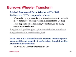
General • bwt: Transforms the order of the symbols of a text. • The bwt output can be very easily compressed. • Used by the compressor bzip2.
Calculating bw(s) • Add an end-of-string symbol ($) to s • Generate a matrix of all the cyclic shifts of s • Sort the matrix rows, in right to left lexicographic order • bw(s) is the first column of the matrix • $ sign is dropped. Its location saved
BWT Example mississippi$ississippi$mssissippi$misissippi$misissippi$missssippi$missisippi$missisippi$mississ ppi$mississi pi$mississip i$mississipp $mississippi mississippi$ssissippi$mi$mississippissippi$missippi$mississi ississippi$mpi$mississipi$mississipp sissippi$missippi$missisissippi$missippi$mississ s = mississipi Sorting the rows of the matrix is equivalent to sorting the suffixes of sr (ippississim) bw(s)= (msspipissii, 3)
BWT Matrix Properties F L • Sorting F gives L • s1=F1 • Fi follows Li in s$ • Equal symbols in L are ordered the same as in F m ississippi $s sissippi$m i$ mississipp is sippi$miss ip pi$mississ i i ssissippi$ mp i$mississi pi $mississip p s issippi$mi ss ippi$missi si ssippi$mis si ppi$missis s
F L ms$spipissii $iiiimppssss ? Reconstructing s • Add $ to get F • Sort F to get L • s1=F1 • Fi follows Li in s$ • Equal order of appearance s= m i s s i
F L ms$spipissii $iiiimppssss Reconstructing s L=sort(F) s=F1 j=1 for i=2 to n { a=# of appearances of Fj in {F1 ,F2 , …Fj } j = index of the a’th appearance of Fj in L s = s + Fj }
What’s good about bwt? • bwt(s) is locally homogenous: • For every substring w of s, all the symbols following w in s are grouped together. mississippi$ssissippi$mi$mississippissippi$missippi$mississi ississippi$mpi$mississipi$mississipp sissippi$missippi$missisissippi$missippi$mississ • These symbols will usually be homogenous.
bwt What’s good about bwt? miss_mississippi_misses_miss_missouri mmmmmssssss_spiiiiiupii_ssssss_e_ioir follow _ follow mi follow mis follow m
Statistical Compression We will discuss lossless statistical compression with the following notations: s = input string over the alphabet: Σ = { a1 , a2 , a3 , …, ah } h = |Σ| n = |s| ni = number of appearances of ai in s. log x = log2x
0 1 e 0 1 a 1 c 0 1 b 1 0 d f Zeroth Order Encoding e 0 a 10 c 111 … Every input symbol is replaced by the same codeword for all its appearances: ai ci Kraft’s Inequality: Output size: Minimum achieved for:
Zeroth Order Encoding • Compressing a string using Huffman Coding or Arithmetic Coding produces an output which size is close to |s|H0(s) bits. • Specifically: • Output size is bounded by |s|H0(s), where: is the Empirical Entropy (zeroth order) of s.
Zeroth order Entropy: Example • n1 = n2 = … = nh : • n1 >> n2, n3 … , nh : • s = mississippi
k-th Order Encoding • The codeword that encodes an input symbol is determined according to that symbol, and its k preceding symbols. • Output size is bounded by |s|Hk(s)bits k-th Order Empirical Entropy of s: ws – A string containing all the symbols following w in s.
k-th order Entropy: Example s = mississippi (k=1) • ms=i H0(i)=0 • is=ssp H0(ssp)=0.92 • ss=sisi H0(sisi)=1 • ps=pi H0(pi)=1
i$ s_ mi mmmmmssssss_spiiiiiupii_ssssss_e_ioir i_ se k-th Order Encoding and bwt • After applying bwt, for every substring w of s, all the symbols following w in s are grouped together: • Did we get an optimal k-th order compressor? • Not yet: • Local homogeneity instead of global homogeneity.
k-th Order Encoding and bwt For example: s=ababababababab…. bwt(s)= abbbbbbbbbbaaaaaaaaa w2 (a) w1 ($) w3 (b) H1(s)=0 (wa=bbb… , wb=aaa…) H0(wi)=0 H0(w1 w2 w3 )=H0(s)=1
MoveToFront Compressing bwt • bwt • Arithmetic coding
MoveToFront Compression • Every input symbol is encoded by the number of distinct symbols that occurred since the last appearance of this symbol. • Implemented using a list of symbols sorted by recency of usage. • Output contains a lot of small numbers if the text is locally homogenous. Transforms local homogeneity into global homogeneity.
MoveToFront Compression Σ = { d,e,h,l,o,r,w } s= h e l l o w o r l d mtf-list= mtf(s)= { w, o, l, e, h, d, r } { h, d, e, l, o, r, w } { e, h, d, l, o, r, w } { l, e, h, d, o, r, w } { o, l, e, h, d, r, w } { d, e, h, l, o, r, w } 2 2 3 0 4 6 1 … Initial list may be either: • Ordered alphabetically • Symbols in order of appearance in the string (need to add it to the output)
bwt0 Compression bwt0(s) arit( mtf( bw(s) ) ) Theorem 1 For any k: (h=size of alphabet)
Notations • x’ = mtf(x) • for a string w over {0,1,2, …, m} define: w01 : w, with all the non-zeros replaced by 1. • x’01 : x’, with all the non-zeros replaced by 1. • Note: |bwt(x)| = |x| |mtf(x)|=|x|
Theorem 1 - Proof Lemma 1 s=s1s2…st , s’=mtf(s). Then
Theorem 1 - Proof • bw(s) can be partitioned into at most hk substrings w1, w2, …, wl such that: • s’=mtf(bw(s)). By Lemma 1: |s|Hk(s) • Using bound on output of Arit:
Lemma 1 - Proof s=s1s2…st , s’=mtf(s). Then Encoding of s’: • For each symbol: is it 0 or not? • For non-zeros: encode one of 1, 2, 3, …, h-1 Note: Ignoring some inter-substrings problems.
Encoding non-zeros of s’ Use prefix code (i ci ): s’’ = pcnz(s’) c1 = 10 c2 = 11 ci = 0 0 0 … 0 0 B(i+1) (i>2) |B(i+1)| - 2 |B(i+1)| |ci| <= 2log(i+1) (|c0| = 0) mi= # occurrences of i in s’.
Encoding non-zeros of s’=mtf(s) For any string s: Sum over all symbols of s Proof Na Occurrences of symbol a in s: p1, p2,…, pNa
Encoding non-zeros of s’ s=s1s2…st • For every i: • Summing for all substrings:
Encoding of s’ • For non-zeros: encode one of 1, 2, 3, …, h-1 No more than bits • For each symbol: Is it 0 or not? Encode s’01
Encoding s’01 • If for every si’01the number of 0’s is at least as large as the number of 1’s: and It follows that: • Otherwise …
Encoding s’01 (second case) • If si’01has more 1’s than 0’s for i=1,2,…l: If there are more 1’s than 0’s in si’01, then It follows that:
Encoding of s’ • For non-zeros: encode one of 1, 2, 3, …, h-1 No more than bits • For each symbol: Is it 0 or not? (Encode s’01 ) No more than bits • Total: (after fixing some inaccuracies) No more than bits
Improvement • Use RLE: bw0RL(s) arit( rle( mtf( bw(s) ) ) ) • Better performance • Better theoretical bound:
Notes • Compressor Implementation: Use blocks of text. Sort using one of: • Compact suffix trees (long average LCP) • Suffix arrays (medium average LCP) • General String sorter (short average LCP) • Search in a compressed text: Extract suffix-array from bwt(s). • Empirical Results…