Download
1 / 26
270 likes | 399 Vues
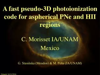
A fast pseudo-3D photoionization code for aspherical PNe and HII regions. C. Morisset IA/UNAM Mexico G. Stasińska (Meudon) & M. Peña (IA/UNAM). H II regions. Where H is photo ionized into H + Need “hot” photons: hot stars (T > 30.000K) PNe Novae Supernovae Active Galactic Nuclei

E N D
A fast pseudo-3D photoionization code for aspherical PNe and HII regions C. Morisset IA/UNAM Mexico G. Stasińska (Meudon) & M. Peña (IA/UNAM)
H II regions • Where H is photoionized into H+ • Need “hot” photons: • hot stars (T > 30.000K) • PNe • Novae • Supernovae • Active Galactic Nuclei • Same processes : same modeling tools • PNe: laboratories for validating the modeling tools
Spherical modeling (1D) • The code computes for each radius (distance to the ionizing source) the ionization and energetic equilibriums, and from there the ionic fractions and emissivities of all the lines. • The geometry is spherical, or plan-parallel (thickness << radius). • This kind of code is developed since the 70’s. • Less than 10 different codes. Public one: Cloudy (G. Ferland). • Regular comparison meeting (benchmarks).
Why photoionization 3D-modeling? • PNe are not spherical : global shape and blobs • Theories: (G)ISW (Kwok), Binarity (Soker), Magnetic field (Corradi): who’s right (if any)? • MHD models in 3D • Velocity fields (access to kinematics)
Short history of 3D photoionization modeling • Viegas & Gruenwald (São Paulo, 1997) • Ercolano (UCL, 2001) : MOCASSIN, Monte-Carlo • Wood & Mathis (2004): Monte-Carlo, a la MOCASSIN • Morisset (IA/UNAM, 2005): NEBU_3D
NEBU_3D • A new pseudo-3D photoionization code (Morisset, Stasińska & Peña, 06/2005, MNRAS). • 1D photoionization code NEBU is run in various directions, the changed parameters being e.g. the inner radius and/or the H-density (but could also be the ionizing radiation: asymmetrical/rotating star). Adaptive in the radial direction. • Reconstruction of a 3D model and visualization/rotation/velocity field, using a set of IDL tools. • Advantages : 1 to 60 minutes to make a model, compared to 30 min / 1 day on cluster for MOCASSIN. • Limitations: diffuse field.
Ellipsoidal PN with knots Density distribution: axy-symetrical, two polar knots. 40 runs of NEBU to be interpolated in a 2003 cube.
« Observational » properties HI HeII [OII] [OIII] • Images in any emission line can be obtained and line intensity variations through any slit.
R([NII]) R([OII]) N+/O+ determination N+/O+ = (I[NII]/e[NII]) / (I[OII]/e[OII]) = (e[OII]/e[NII]) / (I[OII]/I[NII])
Determination of « apparent » parameters • Te, Ne, and N+/O+ are determined along a narrow slit crossing the knot. HI HeII [OII] [OIII]
(N/O) = (N+/O+) N/O = N+/O+? The “apparent” N/O (obtained from N+/O+) is very closed to the “real” value. (N/O) / (N+/O+) However, the 2d-histogram of the values in each cell of the nebula shows that quite no cell has N/O = N+/O+, but on each line of sight, there is quite the same number of cells over- and under- estimating the “true” abundance ratio.
HI HeI [OII] [OIII] Model for a blister HI HeI HI HeI [OII] [OIII] [OII] [OIII] • A blister model is obtained using a plan parallel distribution of the gas, with density increasing outward the ionizing star, a la O’Dell (1995) : NH(z)=NH0 . exp((z-zb)/L) • From a « pole on » point of view, the surface brightness maps are circular, with intensity decreasing with the radius. • The same is obtained with a spherical distribution, the density decreasing with the radial distance to the star : NH(r)=NH0 . exp(-(r/C)²) . B²/(r²+D²). The ionizing star is the same. • This second model is called the « spherical impostor ».
Comparing the blister and its spherical impostor The surface brightness in Hbeta of both models are virtually identical (by construction). Differences exists in low ionization maps.
Comparing the blister and its spherical impostor • The decrease of the “apparent” density observed for the blister model is very similar to the one observed for Orion nebula (O’Dell et al.) • The “apparent” N/O is quite far from the “real” value, especially for the central part of the blister model (SED effects). • See Morisset et al. 2005, MNRAS 360, 499
N/O ≠ N+/O+ • Most of the cells in the data cube are on the y=x bisector (where N/O= N+/O+) • Nevertheless, there is a non negligible amount of cells below this line, leading to a wrong determination of N/O (no compensation as in the PN case).
Velocity fields and line profiles Gesicki & Acker (1993-2003), 3D spherical models for the study of the line profiles. Doesn’t fit the asymmetry of the profiles. The emission line profiles are a kind of convolution between the gas density distribution and the velocity field. The observed complexity of the line profiles is due the complexity of at least one of this two actors.
Emission line profiles produced by NEBU_3D The line profiles are computed trough various apertures, taking into account the thermal broadening, a velocity field (e.g. depending on R, the simplest being Hubble flow) and the turbulence, for each emission lines. Seeing and instrumental profile is also reproduced.
Asymmetrical Profiles from axisymmetrical PNe (NEBU_3D) Complex profiles are obtained using a very simple linear expansion velocity law, and a bipolar density distribution. A small off-center shift for the aperture leads to asymmetrical profiles. Wait for Morisset et al. astroph/xxxx
Hbeta HeII [OII] [OIII]
Use of the line profiles Blister Spherical impostor
Use of the line profiles Turbulence vs. asphericity (line broadening). V=60km/s . R/Rmax V=30km/s . R/Rmax + Vturb (30 km/s) Spherical Nebula, with linear increasing expansion law, without and with turbulence. In this last case, the tails of the profiles are obvious.
Use of the line profiles Turbulence vs. asphericity (line broadening). Only linear expansion law. No Turbulence!!!
What is NEBU_3D not good for? Model of regions where ionization by non-radial continuum is dominant. • Tail of blobs
What is NEBU_3D not good for? Model of regions where ionization by non-radial continuum is dominant. • Tail of blobs • Some 2 components models
Not only PNe • All the tools presented here can be used to model any photoionized region like : • HII regions (blister, etc) • (super) novae expending shells • AGN • star formation regions • Developing a Cloudy_3D…
NEBU_3D Emission line surface brightness maps can be generated for any orientation of the nebula, and can be associated using false color.