Download
1 / 11
110 likes | 128 Vues
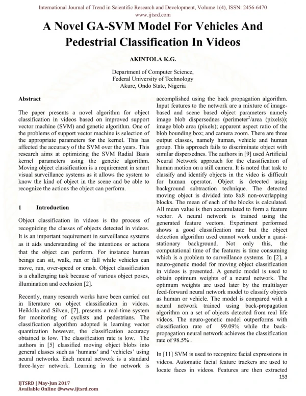
The paper presents a novel algorithm for object classification in videos based on improved support vector machine (SVM) and genetic algorithm. One of the problems of support vector machine is selection of the appropriate parameters for the kernel. This has affected the accuracy of the SVM over the years. This research aims at optimizing the SVM Radial Basis kernel parameters using the genetic algorithm. Moving object classification is a requirement in smart visual surveillance systems as it allows the system to know the kind of object in the scene and be able to recognize the actions the object can perform. This paper presents an GA-SVM machine learning approach for real time object classification in videos. Radial distance signal features are extracted from the silhouettes of object detected in videos. The radial distance signals features are then normalized and fed into the GA-SVM model. The classification rate of 99.39% is achieved with the genetically trained SVM algorithm while 99.1% classification accuracy is achieved with the normal SVM. A comparison of this classifier with some other classifiers in terms of classification accuracy shows a better performance than other classifiers such as the normal SVM, Artificial neural network (ANN), Genetic Artificial neural network (GANN), K-nearest neighbor (K-NN) and K-Means classifiers. Akintola Kolawole G."A Novel GA-SVM Model For Vehicles And Pedestrial Classification In Videos" Published in International Journal of Trend in Scientific Research and Development (ijtsrd), ISSN: 2456-6470, Volume-1 | Issue-4 , June 2017, URL: http://www.ijtsrd.com/papers/ijtsrd109.pdf http://www.ijtsrd.com/computer-science/artificial-intelligence/109/a-novel-ga-svm-model-for-vehicles-and-pedestrial-classification-in-videos/akintola-kolawole-g<br>

E N D
International Journal of Trend in Scientific Research and Development, Volume 1(4), ISSN: 2456-6470 www.ijtsrd.com A Novel GA-SVM Model For Vehicles And Pedestrial Classification In Videos AKINTOLA K.G. Department of Computer Science, Federal University of Technology Akure, Ondo State, Nigeria accomplished using the back propagation algorithm. Input features to the network are a mixture of image- based and scene based object parameters namely image blob dispersednes (perimeter2/area (pixels)); image blob area (pixels); apparent aspect ratio of the blob bounding box; and camera zoom. There are three output classes, namely human, vehicle and human group. This approach fails to discriminate object with similar dispersednes. The authors in [9] used Artificial Neural Network approach for the classification of human motion on a still camera. It is noted that task to classify and identify objects in the video is difficult for human operator. Object is detected using background subtraction technique. The detected moving object is divided into 8x8 non-overlapping blocks. The mean of each of the blocks is calculated. All mean value is then accumulated to form a feature vector. A neural network is trained using the generated feature vectors. Experiment performed shows a good classification rate but the object detection algorithm used cannot work under a quasi- stationary background. computational time of the features is time consuming which is a problem to surveillance systems. In [2], a neuro-genetic model for moving object classification in videos is presented. A genetic model is used to obtain optimum weights of a neural network. The optimum weights are used later by the multilayer feed-forward neural network model to classify objects as human or vehicle. The model is compared with a neural network trained using back-propagation algorithm on a set of objects detected from real life videos. The neuro-genetic model outperforms with classification rate of 99.09% while the back- propagation neural network achieves the classification rate of 98.5% . In [11] SVM is used to recognize facial expressions in videos. Automatic facial feature trackers are used to locate faces in videos. Features are then extracted Abstract The paper presents a novel algorithm for object classification in videos based on improved support vector machine (SVM) and genetic algorithm. One of the problems of support vector machine is selection of the appropriate parameters for the kernel. This has affected the accuracy of the SVM over the years. This research aims at optimizing the SVM Radial Basis kernel parameters using the genetic algorithm. Moving object classification is a requirement in smart visual surveillance systems as it allows the system to know the kind of object in the scene and be able to recognize the actions the object can perform. 1 Introduction Object classification in videos is the process of recognizing the classes of objects detected in videos. It is an important requirement in surveillance systems as it aids understanding of the intentions or actions that the object can perform. For instance human beings can sit, walk, run or fall while vehicles can move, run, over-speed or crash. Object classification is a challenging task because of various object poses, illumination and occlusion [2]. Not only this, the Recently, many research works have been carried out in literature on object classification in videos. Heikkila and Silven, [7], presents a real-time system for monitoring of cyclists and pedestrians. The classification algorithm adopted is learning vector quantization however, the classification accuracy obtained is low. The classification rate is low. The authors in [5] classified moving object blobs into general classes such as ‘humans’ and ‘vehicles’ using neural networks. Each neural network is a standard three-layer network. Learning in the network is 153 IJTSRD | May-Jun 2017 Available Online @www.ijtsrd.com
International Journal of Trend in Scientific Research and Development, Volume 1(4), ISSN: 2456-6470 www.ijtsrd.com which are then supplied to SVM to recognize facial expression. The classification accuracy shows that SVM is capable of recognizing facial expressions. In [12], SVM is used to recognize detected objects in video for tracking purposes. A simple background subtraction technique is used to extract the object. Moment features of the detected objects are calculated and fed into SVM for classification. In [11] and [12] more classification accuracy could have been achieved by optimizing the parameters of the SVM. The hybrid of GA and SVM have been used in [13] for classification of satellite images. There is the need to improve the object classification in video surveillance applications. margin (maximizes the distance between it and the nearest data point of each class). This linear classifier is termed the optimal separating hyper-plane. Intuitively, this boundary is expected to generalize well as opposed to the other possible boundaries. Let m-dimensional training input vectors, xi (i=1,…,m) belong to class 1 or 2 and the associated labels be yi =1 for class 1 and -1 for class 2. If these data are linearly separable, a decision function satisfying Equation 1 can be constructed. b x w x D i ) ( where w is an m-dimensional vector and b is a bias T (1) term. If the training data is linearly separable, then no training data satisfy: Recently SVM have been reported as an efficient classifier. SVM is based on the statistical learning method based on structural risk minimization instead of the empirical risk minimization to improve the generalization ability of a model. It is however realized that the selection of appropriate kernel and kernel parameters can have great influence on the performance of the model [13]. The approach that have been used for optimizing the hyper-parameters of the SVM is the grid search which is always time consuming and does not perform well [13]. In this paper, a genetically optimized support vector machine is presented for human object classification in videos. b T w x 0 (2) i This hyper-plane should have the best generalization capability. As shown in Figure 1, the +1 and the -1 are the training dataset which belong to two classes. The plane H series are the hyperplanes that separate the two classes. The optimal plane H is found by || / 2 w . Hyperplanes || maximizing the margin value H and H are the planes on the border of each class 1 2 and also parallel to the optimal hyper-plane H. The 2 Support Vector Machines (SVM) H and H are called support vectors data located on 1 2 Support Vector Machines are a set of supervised learning methods used regression. This machine learning technique was proposed by Vapnik in 1995. The classification problem can be restricted to consideration of the two- class problem without loss of generality. In this problem, the goal is to separate the two classes by a function which is induced from available examples [16]. The motivation for SVM is to create a classifier that will work well on unseen examples, that is, generalizes well. The objective is to create a classifier that uses the structural minimization principle as against those that use empirical error minimization principle. Consider the example in Figure 1. There are many possible linear classifiers that can separate the data, but there is only one that maximizes the [8]. in classification and Figure 1 The SVM Binary Classification 154 IJTSRD | May-Jun 2017 Available Online @www.ijtsrd.com
International Journal of Trend in Scientific Research and Development, Volume 1(4), ISSN: 2456-6470 www.ijtsrd.com Given a set of training samples m x ,..., x , x 2 1 with labels } 1 , 1 { , a hyper-plane b x w. separates the data into classes such that: 1 if 1 x . w y b i i (4) m j b y y x x (11) i i i i j iy 1 The prediction of new patterns is given by i 1 The training samples for which the Lagrange multipliers are non-zero are called support vectors. Samples for which the corresponding Lagrange multiplier is zero can be removed from the training set without affecting the position of the final hyperplane. The classification framework outlined above is limited to linear separating hyperplanes. It is possible however to use a non-linear hyper-plane by first mapping the sample points into a higher dimensional space using a non-linear mapping. That is, by choosing a map n : is greater than . n A separating hyper-plane is then found in the higher dimensional space. This is equivalent to a non-linear separating surface in The data only ever appears in our training problem in the form of dot products, so in the higher dimensional space the data appears in the form dimensionality of is very large, this product could be difficult or expensive to compute. However, by introducing a kernel function such that: ) ( ). ( ) , ( j i j i K x x x x Equation 13 can be used in place of in the optimization problem and never need to know explicitly what is. The development of a SVM classification model depends on the selection of kernel function K. There are several kernels that can be used in SVM models. These include linear, polynomial, Radial Basis Function (RBF) and sigmoid function. The Radial Basis Kernel is given by: 2 2 The RBF is by far the most popular choice of kernel types used in SVM. This is mainly because of their localized and finite responses across the entire range of the real x-axis. After solving for wand b, the class a test vector w m Class( x ) sign y x x b (12) (3) i i i i k w x . b 1 if y 1 i i i i . These constraints can be expressed in compact form as: ) x . (w b y i i (5) which can be written as: 1 ) x . (w b y i i It has been shown that if no hyper-plane exists (because the data is not linearly separable), a penalty terms This can be translated to the following minimization problem: minimize: where C, the capacity, is a parameter which allows us to specify how strictly the classifier can fit the training data. This can be translated into the following dual problem: i (8) subject to: i which can be solved by standard techniques of quadratic programming. The vector w that defines the optimum separating hyperplane is obtained by: m iy w x . The threshold b of the optimal separating hyper-plane is obtained by: j 1 1 (6) 0 where the dimension of i is added to account for misclassifications. . n (7) . If the ( x ). ( x ) 2 w / 2 C i j i i (13) everywhere x . ix j 1 i , i y y x x maximize: i j i j i j 2 j i 0 C iy 0 i 1 2 (14) K ( x , x ) exp X X i j i 1 i i (9) i m t x belongs to is determined by b or b ) x ( . if a transform to a y x x b y (10) i i i j i t t w. x evaluating 155 IJTSRD | May-Jun 2017 Available Online @www.ijtsrd.com
International Journal of Trend in Scientific Research and Development, Volume 1(4), ISSN: 2456-6470 www.ijtsrd.com higher dimensional space has been used. It can be shown that the solution for w is given by: iy w x (15) takes place, the crossover operator exchanges parts of two single chromosomes to produce children and the mutation operator changes the gene value in some randomly chosen location of the chromosome [10]. The process of evaluation, recombination is iterated until the population converges to an acceptable Algorithms (GA) has been applied in various areas of computer vision such as weights optimization of artificial neural networks segmentation [4]. 3 SVM parameter selection based on Genetic i i Therefore, i selection, and . x w t ) ( b can be rewritten thus: K i solution.Genetic i ) x ( (16) x ( iy ) b iy x ( , x ) b t t i i i i [2;10;14;15], video Thus, the Kernel function can be used rather than actually making the transformation to higher dimensional space since the data appears only in dot Algorithm product form. The σ and C are the free hyper- Using the Genetic algorithm, the two parameters C and σ of SVM model can be optimized. The process of optimizing these parameters is shown in Figure 2. parameters the users can supply. These two parameters has a great role to play in the performance of the SVM. Several choices have used to select Initialization optimal values of these parameters. These include cross-validation, Particle swarm optimization and Train SVM genetic optimization. In this paper, however, the genetic program approach is employed. Calculate fitness by Cross-validation 3 Genetic Algorithm 3.1 Genetic Algorithms Genetic Algorithm (GA) was developed by John Holland in 1975. The algorithm is based on the mechanics of the natural selection process (biological evolution). The concept of the GA is that the strong tends to adapt and survive while the weak tends to die out [17] The technique is about generating a random initial population of individuals, each of which represents a potential solution to a problem [14]. The process begins by coding the genes in a form that represents the solution to the particular problem. In Holland’s Genetic Algorithm, each feasible solution is encoded as a chromosome (string of zeros and ones) also called a genotype. Then initial population size is specified and a number of chromosomes of the population size are then created. Optimization is based on evolution, and the "Survival of the fittest" concept. Each chromosome is given a measure of fitness via a fitness (evaluation or objective) function. The fitness of a chromosome determines its ability to survive and produce offspring [17]. As reproduction Perform Cross Over Perform Mutation No Yes Terminate? Output SVM optimal Figure 2 Flowchart of GA for SVM parameters optimization. a.Initialization. To start with, the initial population is made up of chromosomes chosen at random or based on heuristically selected strings. Population size affects the efficiency of the performance of a GA. The first step in GA implementation is the 156 IJTSRD | May-Jun 2017 Available Online @www.ijtsrd.com
International Journal of Trend in Scientific Research and Development, Volume 1(4), ISSN: 2456-6470 www.ijtsrd.com determination of a genetic encoding scheme, that is, to denote each possible point in the problem’s search space as a characteristic string of defined length. The genes represent the value of σ and C and are concatenated to form a chromosome. Several of these chromosomes are randomly generated from the network architecture to form the initial population of the solution space. Figure 3 shows a typical chromosome. work, the roulette wheel method is adopted for selection. The probability of selection is given by: (19) ? ?? ??= = ???? ? ??? ∑ ?? in which; fi is the fitness value of individual i, fsum is the total fitness value of population; Pi is the selective probability of individual. It is obvious that individuals with high flexibility values are more likely to be reproduced during the next generation. Figure 3: Sample Chromosome Encoding of C and σ of the RBF using strings. 01010 10011 d. one-point crossing is adopted. The specific operation is to randomly set one crossing point among individual strings. When crossing is executed, partial configuration of the anterior point and posterior point are exchanged, and this gave birth to two new offspring Perform Crossover. In this research work, In this research work, C and σ values of the RBF are simultaneously coded as one gene. Each of the gene is coded using randomized binary numbers of length 5. The minimum value is 0.1 while the maximum value is 100. The number of bits to represent the value of a gene must satisfy: e. Mutation. As for two-value code strings, mutation operation is to reverse the gene values within a random number generated between zero and one. Termination Criterion: The termination condition is the maximum number of generations. Genetic control parameters dictate how the algorithm will behave. Changing these parameters can change the computational result. These parameters are population size, crossing probability, mutation probability and network termination condition. In this work population size N is 50, crossing probability Pc is 0.8, mutation probability Pm is 0.5, and network’s terminative condition is MAXGEN of 100. 4 Object Classification using the proposed GA-SVM model ? ≥ ????(????? ??????? ?? + 1);i=1,2.3,, ∆? f. (17) where v is the string length, min?? ?? is the minimum value of the gene, max?? ?? is the maximum value of the gene and ∆? is the error tolerance. A chromosome represents one RBF. The length of chromosome is obtained by concatenating the bits representing each gene as shown in Figure 3. b. When GA is applied to solve a problem, the definition of the evaluation function to evaluate the problem-solving ability of a chromosome is important. Since SVM works by classification, the classification rate is used as the fitness function. The Accuracy is computed as: Accuracy=correctly / total *100 Fitness Function by Cross-Validation. 4.1 The data used for this research work are obtained from videos of moving objects taken in Nigeria roads. The moving objects are detected using background subtraction algorithm and the features are extracted from the silhouettes of the detected objects. 4.1.1 Object Segmentation Data Acquisition (18) c. offspring is calculated and sorted in the descending order. So, chromosomes of highest fitness values are selected for the next generation. In this research Perform Selection. The fitness of the new 157 IJTSRD | May-Jun 2017 Available Online @www.ijtsrd.com
International Journal of Trend in Scientific Research and Development, Volume 1(4), ISSN: 2456-6470 www.ijtsrd.com Kernel Density Estimation (KDE) is the mostly used and studied nonparametric density estimation algorithm. The model is the reference dataset, containing the reference points indexed natural numbered and has been used in [6]for foreground detection. The algorithm assumed that a local kernel function is centered upon each reference point and its scale parameter (the bandwidth). The common choices for kernels include the Gaussian and the Epanechnikov kernel. The algorithm is presented as follows. Let ?? ,?? ,…,??, ϵ ?? be a random sample taken from a continuous, univariate density f, KDE is given by: frames) are used to build histogram of distributions of the pixel color. No classification is done for these learning frames, but for the subsequent frames depending on whether the obtained value exceeds the threshold or not. If the threshold is exceeded, background classification foreground classification. Typically, in a video sequence involving moving objects, at a particular spatial pixel position a majority of the pixel observations would correspond to the background. Therefore, background clusters would typically account for much more observations than the foreground clusters. This means that the probability of any background pixel would be higher than that of a foreground pixel. The pixels are ordered based on their corresponding value of the histogram bin which relies on the adaptive threshold in the previous stage. The pixel intensity values for the subsequent frames are estimated and the corresponding histogram bin is evaluated with the bin value corresponding to the intensity determined. is done, otherwise ??(?,ℎ) = ? ?????? ? ??? ??∑ ?? (20) k(.) is the function satisfying : ??(?)?? = 1 (21) k(.) is refered to as the Kernel, h is a positive number, usually called the bandwidth or window width. The Gaussian Kernel is given by: ??= (2?)?? where r = ‖?‖? ?exp?? ? ?? ? 4.1.2 Feature Extraction (22) The blobs extracted from videos used to extract the feature vectors which were are then normalized by dividing the vector by the sum of the lengths. These vectors are then used to train the support vector machine. The Epanechnikov kernel is given by: ? ? ??(???)(???) ?? ? < 1 0 ??ℎ?????? ??? ??= ? (23) Instead of segmenting the silhouettes into 8x8 non- overlapping blocks as shown in [9], radial features are directly calculated from the detected objects as shown in Figure 4. This captures the shape and a series of the features encodes the motion information. where d is the dimension of feature space, ?? is the volume of the d-dimensional sphere. KDE for background modeling involves using a number of frames (training frames) to build the probability density of each pixel location. The adaptive threshold of each pixel is found after the construction of the histogram. For every pixel observation, classification involves determining if the pixel belongs to the background or the foreground (as shown in Figure 4). The first few initial frames in the video sequence (called learning The centroid of the contour (cx, cy) is calculated using Equation 24. From the centroid, a pre-defined number of axes are projected outwards at specified regular angles to the nearest edges of the contour in an anti- clockwise direction as shown in Figures 4. ? ? (∑ ? ??? ? ??? ,∑ ) ???,??? = (24) ?? ?? 158 IJTSRD | May-Jun 2017 Available Online @www.ijtsrd.com
International Journal of Trend in Scientific Research and Development, Volume 1( International Journal of Trend in Scientific Research and Development, Volume 1(4), ISSN: www.ijtsrd.com ), ISSN: 2456-6470 car features car features 0.1 Figure 4: The radial Distance Shape Features Extraction : The radial Distance Shape Features 0.05 car features Figure 5b: Typiocal Radial 1 vector from Humans (left) and vehicles (right) 0 1 5 9 1317212529 29 The distance from the centroid to its nearest edge along a predefined angle is then stored. This is done for a set of angular vectors. The dimension of each vector equals the number of axes being projected the centroid. The vector is then normalized to ensure that the vector is scale invariant and the largest value in the vector will at this point be 1.0, which will be the longest of the axes projected. Figure show the execrated features from human and vehicles respectively. The distance from the centroid to its nearest edge along a predefined angle is then stored. This is done for a set of angular vectors. The dimension of each vector equals the number of axes being projected from the centroid. The vector is then normalized to ensure that the vector is scale invariant and the largest value in the vector will at this point be 1.0, which will be the longest of the axes projected. Figures 5a and 5b features from human and vehicles : Typiocal Radial 1- D distance feature vector from Humans (left) and vehicles (right) be the segmented object region within the be a line projected from the centroid to the to the horizontal line passing through the centoroid of the object, then the length of each line to the contour boundary of the Let S be the segmented object region within the frame, ?? be a line projected from the centroid to the object boundary at angle i passing through the centoroid of the object, then the length of each line to the contour boundary of the object is given by: ? ??? ?? = ∑ ?(?(?,?)) (25) k and l are the co-ordinates in the respectively c is the centre point and boundary. l is given by ktan( function that returns 0 or 1. ordinates in the x and y directions is the centre point and w is the contour is given by ktan(?), ?(.) is a binary human features ???(?,?)? = ? 1 ?? ?(? (?,?) ? ? ?????? (26) 0.06 0 ??ℎ?????? 0.04 human features 0.02 where p(k, ?) is the pixel value of the object. ) is the pixel value of the object. 0 The number of lines in each image containing an object as well as the number of neurons in the input layer is j where j = 1, 2, 3, …., n and n is given by n = is the smallest of the angles. Angular size of 10 degrees interval is used to obtain 36 regions beginning with 100. Thirty two (32) of were selected as feature vectors. See [1] The number of lines in each image containing an object as well as the number of layer is j where j = 1, 2, 3, …., n and n is given by n = 360/???? where ???? is the smallest of the angles. Angular size of 10 degrees interval is used to obtain 36 regions beginning with 10 these regions were selected as feature vectors. for more details of the segmentation algorithm. for more details of the segmentation algorithm. 1 5 9 13 17 21 25 29 Figure 5a: Typiocal Radial 1- D distance feature vector from Humans (left) and vehicles vector from Humans (left) and vehicles (right) D distance feature 159 IJTSRD | May-Jun 2017 Available Online @www.ijtsrd.com
International Journal of Trend in Scientific Research and Development, Volume 1(4), ISSN: 2456-6470 www.ijtsrd.com GA-SVM Object Classification compare the classification performance of the proposed model with other classifiers such as the normal SVM, K-Means, K-NN, ANN, GA-ANN, the training is done with the same set of data and the same testing dataset is used to evaluate each classifier. In the proposed GA-SVM model, the SVM adopts Radial Basis Function as the kernel. The parameters C and γ of the SVM are optimized using Genetic Algorithm. Then these optimal parameters are used to train the SVM model. In the normal SVM model, the SVM use RBF as the kernel function. The parameters C and γ are randomly selected. In the K-Nearest Neighbour training, data for vehicles and pedestrians are provided for the K-NN. As many instances of vehicles and pedestrians are provided with their corresponding class labels. After the training is done, K-Nearest can then be used to classify test instances. To classify a new instance, the instance is supplied and the number of neighbors k. This k defines the neighborhood in which training data is consulted. The test data is compared with the training data. The nearest K-instances are checked and the majority nearest to k dictates the class that the instance belongs. In this research, k is set to 5. For the Classification Using K-Means Algorithm, Given a training set of human and vehicle classes, a K-Means clustering algorithm is trained using the vector X = (x1, x2,...,xL) for human and Y = (y1,y2, ..., yL) for vehicle data. where L is the total number of training images. To train the K-means, the number of classes and the mean of each class is provided. K-Means now clusters each data item to any of the classes based on the Euclidean distance of the data to the mean of each cluster. The minimum distance from each class determines which cluster the data falls. Now after the entire instance are clustered, the means are re- evaluated again and the process continues until a given terminating condition is fulfilled. To cluster a new data, the distances of the new data to each of the evaluated cluster means are calculated and the one with minimum is the class of the new data. Object classification using ANN uses input nodes, which are 32 in number, the hidden layer which has 32 neurons and the output layer which has one neuron. The following steps are adopted in the Neural Network modeling for object classification. In this approach, shape features extracted from the detected moving objects are used to train a neural network classifier in order to recognize human and vehicle classes. The Learning Algorithm used is the back propagation algorithm. The dimension of input data is thirty two. 4.2 In this work, the training of the SVM consists of providing the SVM with data for vehicles and pedestrians. Data for each class consist of a set of n dimensional vectors. A Radial Basis Function (RBF) kernel is applied to the SVM which then attempts to construct a hyper-plane in the n- dimensional space, attempting to maximize the margin between the two input classes. The SVM type used in this work is C-SVM using a non-linear classifier where C is the cost hyper-parameter [2]. The SVM is trained using 1D radial signals extracted from the silhouettes of the labeled images of humans and vehicles. Given a training set of human and vehicle images consisting of multiple labeled images of each human and vehicle classes an SVM classifier is trained as follow: 1D features data are extracted from the training set images to create the vector X = (x1, x2,...,xL) for human and Y = (y1,y2, ..., yK) for vehicle images. where L and K are the total number of training images for class human and vehicle respectively. To train the SVM, X = (x1, x2, ..., xL) are used as the positive labeled training data and Y = (y1,y2, ...,yL) are used as the negative labeled training data. The SVM is then trained to maximize the hyper- plane margin between their respective classes (Φ1, Φ2). To classify an object F, it must be assigned to one of the p possible classes (Φ1, Φ2), in this case p takes two values. For each object class, Φp, an SVM is used to calculate this class that the object F belongs to given measurement vector D where in this case D is the set of 1D radial features. 5 Implementation of the Proposed Model In order to evaluate the classification performance of the proposed SVM model, some video data were gotten from major roads in Akure, Nigeria. The background subtraction algorithm was applied to detect objects from the videos. Features of these objects are exccted and stored in a database. The data are divided randomly into the 80 training dataset 333 test dataset. The 80 training dataset consist of 40 vehicles and 40 pedestrians. The test dataset consists of 100 vehicles and 223 pedestrians. The class vehicle is assigned 1 while the class human is assigned 0. The GA-SVM model is trained using [3]. In order to 160 IJTSRD | May-Jun 2017 Available Online @www.ijtsrd.com
International Journal of Trend in Scientific Research and Development, Volume 1( International Journal of Trend in Scientific Research and Development, Volume 1(4), ISSN: www.ijtsrd.com layer having thirty two neurons and one output neuron. The network is . This is a supervised learning algorithm in which the input vectors are supplied together with the desired output. The back propagation algorithm (BPN) learns during the training epoch. Several epochs are needed before the network can sufficiently learn and provide a The number of epochs used is 500, with the momentum of 0.5 and learning rate of y initialized to small random numbers less than 1 using random The object classification using ANN) applies genetic algorithm to optimize the weights before the ANN is In this case, there which signifies a opulation size N is 50, crossing mutation probability Pm is 0.015 and network’s terminative condition is MAXGEN of n excellent empirical ), ISSN: 2456-6470 The network has one hidden layer having thirty two neurons and one output neuron. The network is trained using the back-propagation. supervised learning algorithm in which the input vectors are supplied together with the desired output. The back propagation algorithm (BPN) the training epoch. Several epochs are needed before the network can sufficiently learn and provide a satisfactory result. The number of epochs used is 500, with the momentum of 0.5 and learning rate of 0.3. The initial weights are randomly initialized to small random numbers less than 1 using random number generators. The object classification using using neuro-genetic model (GA-ANN) applies genetic algorithm to optimize the weights before the ANN is trained with the optimized weight. In this case, there are (32*32+32) number of weights which signifies a chromosome. The population size N is 50, crossing probability Pcis 0.8, mutation probability and network’s terminative condition is MAXGEN of 100. This combination gives an excellent empirical performance. S PARAME GA S GA K- A K- N TER - V - ME N N SV M AN AN N N M N S 1 Number 413 41 41341341 41 observed 3 3 3 features 2 Number of 80 80 80 80 80 80 training set 3 Number of 2 2 2 2 2 2 classes 4 Dimension 32 32 32 32 32 32 of input features 5 Number of 333 33 33333333 33 test set 3 3 3 6 Results and discussion 6 Total 331 33 330 329 32 31 Table 1 shows the analysis result for SVM,GA-ANN, K-MEANS, K-NN. GA the GA-SVM, 80 data are used to train the model. The support vectors’ values from the training are then saved. The gamma parameter obtained is 19.28 and the C value is 6.49. For testing, 333 consisting of 110 vehicle data and 223 pedestrian data are used. Out of the 110 vehicles, all are classified correctly while for 223 human class data items, o are misclassified. Error in classification the accuracy is 99.39%. For the normal classification is 0.9% and the accuracy is 99.1%. For GA-ANN, error in classification is 0.9% and the accuracy is 99.1%. For K-MEANS classification is 1.2% and the accuracy is 98.8% and for ANN, error in classification is 1.5% and accuracy is 98.5% and for K-NN, error in classification and accuracy is 95.2%. Figure 6 classification accuracy. From the figure, it is show that the proposed model has the highest classification accuracy. Table 1 Comparison of Classification Algorithms the analysis result for GA-SVM, NN. GA-SVM. For SVM, 80 data are used to train the model.. The support vectors’ values from the training are then The gamma parameter obtained is 19.28 and For testing, 333 data items Recognize 0 8 7 d Classificati 99. 99 99. 98. 98 95 7 on 39 .1 1% 8% .5 .2 pedestrian data accuracy % % % % . Out of the 110 vehicles, all are classified correctly while for 223 human class data items, only 2 classification is 0.61% and the normal SVM, error in is 0.9% and the accuracy is 99.1%. For 100.00% is 0.9% and the MEANS, error in 99.00% 98.00% is 1.2% and the accuracy is 98.8% and is 1.5% and accuracy classification is 4.8% 97.00% 96.00% Series1 95.00% 6 shows the 94.00% accuracy. From the figure, it is showned that the proposed model has the highest classification 93.00% K-MEANS ANN ANN SVM K-NN GA-ANN GA-SVM 1 Comparison of Classification Algorithms Figure 6: Classification Accuracy of the classifiers Accuracy of the classifiers 161 IJTSRD | May-Jun 2017 Available Online @www.ijtsrd.com
International Journal of Trend in Scientific Research and Development, Volume 1(4), ISSN: 2456-6470 www.ijtsrd.com [5] Collins, R. T., Lipton, A. J., Fujiyoshi, H., and Kanade, T. (2000). A System for Video Surveillance and Monitoring: VSAM Final Technical Report, Robotics Institute, University, May 2000. 7 Conclusion In this paper, SVM with GA is applied to object classification in videos. In the proposed model, an optimized RBF kernel function and parameter C of SVM is obtained. Video data of moving objects have been used to evaluate the model. The experimental results show that the proposed classifier performs better than the SVM in which parameters are chosen randomly. The comparative analysis of the model with that of SVM, GA-ANN, K-MEANS, K- NN.ANN shows that the model shows more excellent performance in terms of classification accuracy. In future other optimization techniques will be looked into in order to investigate the performance of the SVM model on other optimization techniques. CMU-RI-TR-00-12, Carnegie Mellon [6] Elgammal A., Duraiswami R, Harwood D.,and Davis L.S. (2002). Foreground Modeling Using Nonparametric Kernel Density Estimation Surveillance. Proceedings of the IEEE Vol.90, No.7, pp. 1151-1163, JULY 2002. Background and for Visual [7] Heikkila J. and Silven O. (1999) A real-time system for monitoring of cyclists and pedestrians. Prococeedings of Second IEEE Workshop on Visual Surveillance, pp. 74–81, Fort Collins, Colorado, June 1999. References [1] [8] Hochreiter Bioinformatics and Machine Learning Lecture Notes. Institute of Bioinformatics, Johannes Kepler University A-4040 Linz, Austria. [9] Modi R. V. and Mehta T. B. (2011). ‘Neural Network-Based Approach for Recognition of Human Motion Using Stationary Camera’. International Journal Applications, Vol. 25, No. 6, pages 975-887. [10] Montana D.J., and Davis L.D. (1989). Training Feed-Forward Genetic Algorithms. Proceedings of the International Joint Conference on Artificial Intelligence, IJCAI-89. Morgan Kaufman Publishers, Deutrot, MI, pp.762-767. [11] Michael P. and El-Kaliouby R. (2003) Real time facial expression recognition in video using Support Vector Machine in proceedings of ICM Nov 5-7, 2003 Vancour, British Columbia, Canada. [12] Ramya G and Srclatha M. (2014) Multiple Object Tracking using Support Vector Machine. Global Journal of Researches in Engineering Subtraction Vol. 14 Issue 6 Version 1. S., (2009). Theoretical Akintola K.G, Tavakkolie A. (2011). Robust Foreground Detection in Videos using Adaptive Colour Histogram Thresholding and Shadow Removal. Proceedings of the 7th International Symposium Computing, Vol. part ii JSVC’11, pp. 496-505, Berlin, Heideiberg, Germany, September, 2011. on Visual of Computer [2] Akintola K.G., Olabode O. (2014) A Neuro- Genetic Model For Classification In Video Surveillance Systems. International Journal of research in Computer Applications and Robotics Vol. 2, No8 pp. 143-151, July, 2014. Moving Object Networks using [3] Chang C.C and Lin, C. J. (2001) LIBSVM: A Library for Support Software available at http://www.csie.ntu.edu.tw/~cjlin/libsvm. Vector Machines. [4] Chiu P., Girgensohn A., Polak W., Rieffel, E, Wilcox L. (2000). A Genetic Algorithm for video Segmentation and Summarization. Proceedings of IEE International Conference on Multimedia and Expo, Vol. 3, pp. 1329- 1332, New York, 30th July-2nd August, 2000. 162 IJTSRD | May-Jun 2017 Available Online @www.ijtsrd.com
International Journal of Trend in Scientific Research and Development, Volume 1(4), ISSN: 2456-6470 www.ijtsrd.com [13] Ravindra M Chandraslekhar G. (2014) Classification of Satellite Images based on SVM Classifier using International Journal of Innovative Research in Electrical Electronics Instrumentation and Control Engineering Vol. 2 Issue 5, May 2014 [14] Rilley J., Ciesielski V.B. (1998). An Approach to Training Feed-Forward and Recurrent Neural Networks. Proceedings of the Second International Conference on Knowledge-Based Intelligent Electronic Systems (KES’98), pp. 596-602, Adelaide, April 1998, USA. [15] VishwaKarma D.D. Algorithm Based Weights Optimization of Artificial Neural Network, International Journal of Advanced Research in Electrical, Electronics and Instrumentation Vol. 1. No 3, August 2012. [16] Vapnik V,N.(1995). The Nature of Statistical Learning Theory. Springer Verlag, New York, 1995. ISBN, 0-387-94559-8. [17] Wainwright R.L. (1993). Introduction to Genetic Algorithms Theory and Applications. The seventh Oklahoma Symposium on Artificial Intelligence. November, 19,1993. The University of Tilsa Cao Smith College Avenue, Tulsa Oklaoma. Genetic Algorithm. (2012). Genetic 163 IJTSRD | May-Jun 2017 Available Online @www.ijtsrd.com