Topics Telecon - Dec 18
550 likes | 684 Vues
Topics Telecon - Dec 18. Review Cheryl’s dissertation proposal slides: ignore “Results” section for now (will replace this with more organized results set, primarily based on IEPC 09 run) Need help with slide 6 – relevant Hall thruster simulations Additional comments on slides 5 and 7?

Topics Telecon - Dec 18
E N D
Presentation Transcript
TopicsTelecon - Dec 18 • Review Cheryl’s dissertation proposal slides: ignore “Results” section for now (will replace this with more organized results set, primarily based on IEPC 09 run) • Need help with slide 6 – relevant Hall thruster simulations • Additional comments on slides 5 and 7? • Wall loss model – review notes sent by Eduardo • Upwind discretization – turned “on/off” in the code? • Research plan: slides 45-52 – seems ambitious, need help with prioritization/goals • IEEE TPS paper edits – Thanks, Eduardo!
AXIAL-AZIMUTHAL HYBRID FLUID-PIC SIMULATIONS OF COHERENT FLUCTUATION-DRIVEN ELECTRON TRANSPORT IN A HALL THRUSTER Cheryl M. Lam Advisor: Mark A. Cappelli Stanford Plasma Physics Laboratory Mechanical Engineering Department Dissertation Proposal Meeting December 20, 2013
Dissertation Outline • Introduction • Hall Thruster Simulations (Background) • Model Description: Hybrid Fluid-PIC z-θ Model • Model Sensitivities • Simulation Results • Discussion • Conclusions and Future Work
Hall Thruster • Electric space propulsion device • Demonstrated high thrust efficiencies • Up to 60% (depending on operating power) • Deployed production technology • Design Improvements • Better physics understanding • Basic Premise: Accelerate heavy (positive) ions through electric potential to create thrust • E x B azimuthal Hall current • Radial B field (r) • Axial E field (z) • Ionization zone (high electron density region) • Electrons “trapped” • Neutral propellant (e.g., Xe) ionized via collisions with electrons Plasma • Ions accelerated across imposed axial potential (Ez / Φz) & ejected from thruster
Motivation • Hall thruster anomalous electron transport • Super-classical electron mobility observed in experiments1 • Theory: Correlated (azimuthal) fluctuations in ne and uez induce super-classical electron transport • 2D r-z models use tuned mobility to account for azimuthal effects2,3 • 3D model is computationally expensive • First fully-resolved 2D z-θ simulations of entire thruster ** Initial development by E. Fernandez • Predict azimuthal (ExB) fluctuations • Quantify impact on electron transport Channel Diameter = 9 cm Channel Length = 8 cm 1Meezan, N. B., Hargus, W.A., Jr., and Cappelli, M. A., Physical Review, Vol. 63, No. 2, 026410, 2001. 2Fife, J. M., Ph.D. Dissertation, Massachusetts Inst. of Technology, Cambridge, MA, 1999. 3Fernandez et al, “2D simulations of Hall thrusters,” CTR Annual Research Briefs, Stanford Univ.,1998.
Hall Thruster Simulations • 2D radial-axial (r-z) simulations • Fife • Michelle • Eunsun? – ongoing • 2D axial-azimuthal (z-θ) • Aaron • Mine • French (Garrigues, Bouchoule, Adam, et al.) – not full azimuth • Italian (Taccogna, Cappitelli?) • 3D • Cite recent work – fully-kinetic (PIC) computationally expensive: smaller geometry (smaller-scale thruster) and/or shorter runs • Review IEPC 2013 papers
Relevance of Hybrid z-θ Simulations • Thruster geometry • Scale (thruster size) • Resolve full azimuth • No artificial introduction of periodicity • Time scales of interest • Hybrid approach enables longer (~100s μs) simulations • Low to mid-frequency waves (~10 kHz – 100 MHz?? More like ~MHz because inertialess?)
Channel Diameter = 9 cm Channel Length = 8 cm Anode Cathode Anode Exit Plane extends 4 cm past channel exit z: 40 points, non-uniform θ: 50 points, uniform Geometry • 2D in z-θ • No radial dynamics • E x B + θ • Br: purely radial (measured from SHT laboratory discharge) • Imposed operating voltage (based on operating condition) G G
Hybrid Fluid-PIC Model • Ions: Particle-In-Cell approach • Non-magnetized • No particle-particle collisions; Wall collisions modeled in some cases • Neutrals: Collisionless particles (Particle-In-Cell approach) • Injected at anode per mass flow rate • No particle-particle collisions; Wall collisions modeled in some cases • Ionized per local ionization rate • Based on fits to experimentally-measured collision cross-sections, assuming Maxwellian distribution for electrons • Electrons: Fluid continuum • Continuity (species & current) • Momentum • Drift-diffusion equation • Inertial terms neglected • Energy (1D in z) • Convective & diffusive fluxes • Joule heating, Ionization losses, Effective wall loss Quasineutrality: ni = ne
Interpolation: Particle Grid rNW rNE FNW FNE rSE FSE rSW FSW Interpolation: Grid Particle PIC Ions & Neutrals • Particle-In-Cell (PIC) Approach • Particles: arbitrary positions • Force Particle acceleration Interpolate: Grid Particle • Plasma properties evaluated at grid points (Coupled to electron fluid solution) • Interpolate: Particle Grid • Bilinear Interpolation • Ions subject to electric field: ≈ 0 neglect
Ionization rate • Nu_en • nedot • Neutral injection • Injection velocity: slow vs “normal” (thermalized) • Wall collisions • Neutral particles reflected upon collision with anode or inner/outer radial channel walls • Ions recombine (with donor electron) to form neutral upon collision with inner/outer radial channel walls • Particles still otherwise collisionless, i.e., we do not model particle-particle collisions
Electron Fluid Equations • Species Continuity • Current Continuity 0 ni = ne
Electron Fluid Equations Classical Mobility • Momentum: Drift-Diffusion • Neglect inertial terms Classical Diffusion
Electron Fluid Equations Momentum: Drift-Diffusion Neglect inertial terms Classical Mobility Classical Diffusion E x B classical diamagnetic classical E x B diamagnetic θ fluctuations/dynamics
Electron Fluid Equations Combine current continuity and electron momentum to get convection-diffusion equation for Φ: where (φ is electric potential)
Electron Fluid Equations Energy (Temperature) Equation 1D in z where with ionization cost factor αi = 1 (simplest model)
LEAP FROG Time Advance Particle Positions & Velocities Neutrals & Ions (subject to F=qE) EGRID EPART Ionize Neutrals Inject Neutrals Calculate Plasma Properties ni-PART, vi-PART, nn-PART, vn-PART ni-GRID, vi-GRID, nn-GRID, vn-GRID QUASINEUTRALITY: ne = ni = nplamsa Spline RK4 Time Advance Te=Te(ne, ve) DIRECT SOLVE 2nd-order F-D Iterative Solve Φ Calculate Φ=Φ(ne, vi-GRID) ↔ EGRID Calculate ve=ve(Φ, ne, Te) r < ε0 CONVERGED r = Φ – Φlast-iteration Calculate vi-GRID-TEST= vi-GRID(EGRID) Solution Algorithm Boundary Conditions: • Dirichlet in z (Φ,Te) • Periodic in θ
Model Sensitivities • Grid – current non-conservation • ICs and BCs • Numerical stability/sensitivity of energy (Te) equation • Source/Sink terms • Ionization cost factor • Constant factor • Dugan model • Energy loss to wall
Sample Results • IEPC 2009 runs • Build upon these • More recent – with inclusion of wall collisions?? • IEPC2013 – spoke, do not understand • Higher voltage – do not understand
40 points non-uniform in z 50 points uniform in θ Previous 100V (IEPC 2009) 160V simulation (new) 61 points uniform in z 25 points uniform in θ 100V simulation (new) Numerical Grid
Plasma Density Electron Temperature Axial Ion Velocity Electric Potential Time-Averaged Plasma Properties
E x B Fluctuations Axial Electron Velocity Distinct wave behavior observed: • Near exit plane (as before) • Tilted: + z, - ExB • Higher frequency, faster moving, shorter wavelength • Transition to standing wave (purely +z) downstream of exit plane (z = 0.1 m) • Mid-channel • Tilted: - z, + E x B • Lower frequency, slow moving, longer wavelength • “More tilted” (stronger/faster θ component) – compared to previous • Near anode • Rotating spoke • m = 2 (100V)
Anode Cathode E x B Rotating Spoke • Near anode (z ≤ 0.01 m) • Primarily azimuthal • m = 2 • vph = ~ 1 km/s • f = 10-20 kHz
Correlated ne and uez fluctuations generate axial electron current Uncorrelated Correlated fluctuations generate axial current
Electron Transport Axial Electron Mobility:
Electron Transport • Preliminary Simulation: Spoke does not lead to anomalous transport Axial Electron Mobility:
Rotating Spoke – IEPC13 100V case • Near anode (z ≤ 0.01 m) • Primarily azimuthal • m = 2 • vph = ~ 1 km/s • f = 10-20 kHz
E x B Anode Cathode E x B E x B Fluctuations in θ – IEPC09?? Or 13? f = 40 KHz λθ = 5 cm vph = 4000 m/s f = 700 KHz λθ = 4 cm vph = 40,000 m/s
Streak Plots – IEPC09?? Or 13? E x B E x B
160V SimulationElectron Transport Spoke does not lead to anomalous transport Axial Electron Mobility:
Electron Fluid Equations Momentum: Drift-Diffusion Neglect inertial terms Correlated azimuthal fluctuations induce axial transport: Classical Mobility Classical Diffusion E x B classical diamagnetic classical E x B diamagnetic Previous models under-predict Jez=qneuez θ fluctuations/dynamics
ξ t Azimuthal Fluctuations induce Axial Transport Eθ= E0cos(ωt) ne = n0cos(ωt + ξ) Consider Induced Current Induced current depends on phase shift ξ
Correlated ne and uez fluctuations generate axial electron current Uncorrelated Correlated fluctuations generate axial current
Fluctuations • Compare to experiments • Linearized dispersion relations? • Future results: include dispersion analysis/maps
Anomalous current • Contributions (from various terms) to electron current • Axial variation • Relate to shear, other gradients? • Electron transport / anomalous current – trends with operating conditions (e.g., increased voltage)
Anomalous electron transport • Suggestions for future work • FV? • Fully kinetic simulations
Recent Progress & Challenges • Addition of particle collisions with thruster walls • Neutral particles reflected upon collision with anode or inner/outer radial channel walls • Ions recombine (with donor electron) to form neutral upon collision with inner/outer radial channel walls • Particles still otherwise collisionless, i.e., we do not model particle-particle collisions • Finer axial (z) grid resolution near anode • Stability challenges • Sensitivity to Initial Conditions and Boundary Conditions • Strong fluctuation in Te • Current conservation • Finite Difference – present model • Finite Volume
Additional Simulations – 100V • Establish stable long-running simulation (~600 μs – 1 ms) for low voltage (100V) case • Start from (continue) IEPC 2009 simulation • Ionization cost factor = 1 • No wall collisions; Slow neutral injection velocity • Zero-slope BC for Te • Increase number of particles (ionizspc) to enable longer simulation • Grid refinement study • Finer grid in z: current non-conservation, structure near anode • Finer, varied grid in theta: impact periodicity, azimuthal wavelength? • Initial Conditions • Increased neutral density spoke at anode? • Shape of neutral density profile (peaked/sloping, by how much) • More realistic plasma (electron/ion) density profile and/or magnitude
Additional Simulations – Higher Voltage • Higher voltage runs • Incrementally increase operating voltage • Look for trends (in frequency/wavelength/direction of fluctuations, electron transport, anomalous contribution to transport) • Initial Conditions – Waves • Smooth initial profiles (based on prescribed profile or experiment) – allow fluctuations to evolve (as before) • If needed, of interest, “seed” with particular waves/modes
Development Process • Establish stable low voltage (100 V run) • Increase operating voltage – with all other conditions same as for 100V case • Adjustments as needed to establish stable higher voltage run • Changes to 100V case – model improvements, additional physics, etc. • Establish stable 100V run • Increase operating voltage – with all other conditions same as for 100V case • Adjustments as needed to establish stable higher voltage run • REPEAT
Model Improvements • Te stability and BC/IC impacts • Stability and sensitivity analysis – contribution of source/sink terms, esp. wall loss and ionization cost • Enforcement of (IC/return to) experimental profile and/or experimental-based limits • Prescribed (fixed value) vs. zero-slope condition at domain boundaries • Ionization cost factor • Dugan model • Tuned constant factor? • Improved/tunable wall loss model • Introduction of diffusive damping term? • Effect of spline smoothing • Implicit solve? • Improve stability – consider more global changes to model • “External” power supply circuit model (potential BC) • Hyperviscous damping (for potential equation)
Model Improvements • Incremental changes (additions) to model – additional physics • Introduction of wall collisions (w/ higher thermal injection velocity) • Revisit ionization rate implementation? • Electron transport/mobility – sustain/generate waves (also help stability) • Additive “baseline” mu_perp or nu_en • Experimental mobility (in lieu of or in addition to mu_perp) • Experimental or additional (or Bohm-like) mobility for electron fluid equations only