Download
1 / 54
620 likes | 1.83k Vues
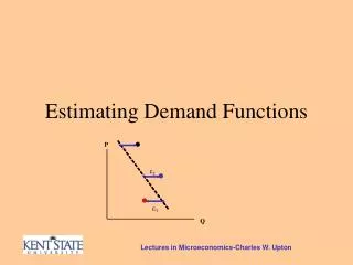
Estimating Demand. Outline Where do demand functions come from? Sources of information for demand estimation Cross-sectional versus time series data Estimating a demand specification using the ordinary least squares (OLS) method. Goodness of fit statistics. . The goal of forecasting.

E N D
Estimating Demand • Outline • Where do demand functions come from? • Sources of information for demand estimation • Cross-sectional versus time series data • Estimating a demand specification using the ordinary least squares (OLS) method. • Goodness of fit statistics.
The goal of forecasting To transform available data into equations that provide the best possible forecasts of economic variables—e.g., sales revenues and costs of production—that are crucial for management.
Demand for air travel Houston to Orlando Recall that our demand function was estimated as follows: Now we will explain how we estimated this demand equation [4.1] Q = 25 + 3Y + PO – 2P Where Q is the number of seats sold; Y is a regional income index; P0 is the fare charged by a rival airline, and P is the airline’s own fare.
Questions managers should ask about a forecasting equations • What is the “best” equation that can be obtained (estimated) from the available data? • What does the equation not explain? • What can be said about the likelihood and magnitude of forecast errors? • What are the profit consequences of forecast errors?
How do get the data to estimate demand forecasting equations? • Customer surveys and interviews. • Controlled market studies. • Uncontrolled market data.
Campbell’s soup estimates demand functions from data obtained from a survey of more than 100,000 consumers
Survey pitfalls • Sample bias • Response bias • Response accuracy • Cost
Types of data Time -series data: historical data--i.e., the data sample consists of a series of daily, monthly, quarterly, or annual data for variables such as prices, income , employment , output , car sales, stock market indices, exchange rates, and so on. Cross-sectional data: All observations in the sample are taken from the same point in time and represent different individual entities (such as households, houses, etc.)
Estimating demand equations using regression analysis Regression analysis is a statistical technique that allows us to quantify the relationship between a dependent variable and one or more independent or “explanatory” variables.
Y Regression theory X and Y are notperfectly correlated.However, there is on average a positive relationshipbetween Y and X 0 X1 X2 X
We assume that expected conditional values of Y associated with alternative values of X fall on a line. Y E(Y |Xi) = 0 + 1Xi Y1 1 1= Y1 - E(Y|X1) E(Y|X1) 0 X1 X
Specifying a single variable model Our model is specified as follows: Q = f (P)where Q is ticket sales and P is the fare Q is the dependent variable—that is, we think that variations in Q can be explained by variations in P, the “explanatory” variable.
Estimating the single variable model Since the datapoints are unlikely to fallexactly on a line, (1)must be modifiedto include a disturbanceterm (εi) [1] [2] • 0 and 1 are called parameters or population parameters. • We estimate these parameters using the data we have available
is the estimated value of y for a given x value. Estimated Simple Linear Regression Equation • The estimated simple linear regression equation • The graph is called the estimated regression line. • b0 is the y intercept of the line. • b1 is the slope of the line.
Sample Data: x y x1 y1 . . . . xnyn Estimated Regression Equation Sample Statistics b0, b1 Estimation Process Regression Model y = b0 + b1x +e Regression Equation E(y) = b0 + b1x Unknown Parameters b0, b1 b0 and b1 provide estimates of b0 and b1
^ yi = estimated value of the dependent variable for the ith observation Least Squares Method • Least Squares Criterion where: yi = observed value of the dependent variable for the ith observation
Least Squares Method • Slope for the Estimated Regression Equation
_ _ x = mean value for independent variable y = mean value for dependent variable Least Squares Method • y-Intercept for the Estimated Regression Equation where: xi = value of independent variable for ith observation yi = value of dependent variable for ith observation n = total number of observations
Line of best fit The line of best fit is the one that minimizes the squared sum of the vertical distances of the sample points from the line
The 4 steps of demand estimation using regression Specification Estimation Evaluation Forecasting
Table 4-2 Ticket Prices and Ticket Sales along an Air Route
Simple linear regression begins by plotting Q-P values on a scatter diagram to determine if there exists an approximate linear relationship:
A v e r a g e O n e - w a y F a r e D e m a n d c u r v e : Q = 3 3 0 - P 5 0 1 0 0 1 5 0 N u m b e r o f S e a t s S o l d p e r F l i g h t Scatter plot diagram with possible line of best fit $ 2 7 0 2 6 0 2 5 0 2 4 0 2 3 0 2 2 0 0
Note that we use X to denote the explanatoryvariable and Y is the dependent variable.So in our example Sales (Q) is the “Y” variable and Fares (P) is the “X” variable. Q = Y P = X
Computing the OLS estimators We estimated the equation using the statistical software package SPSS. It generated the following output:
Reading the SPSS Output From this table we see that our estimate of 0 is 478.7 and our estimate of 1 is –1.63. Thus our forecasting equation is given by:
Step 3: Evaluation • Now we will evaluate the forecasting equation using standard goodness of fit statistics, including: • The standard errors of the estimates. • The t-statistics of the estimates of the coefficients. • The standard error of the regression (s) • The coefficient of determination (R2)
Standard errors of the estimates • We assume that the regression coefficients are normally distributed variables. • The standard error (or standard deviation) of the estimates is a measure of the dispersion of the estimates around their mean value. • As a general principle, the smaller the standard error, the better the estimates (in terms of yielding accurate forecasts of the dependent variable).
The following rule-of-thumb is useful: The standard error of the regression coefficient should be less than half of the size of the corresponding regression coefficient.
Computing the standard error of 1 Let denote the standard error of our estimate of 1 Note that: Thus we have: and Where: and k is the number of estimated coefficients
By reference to the SPSS output, we see that the standard error of our estimateof 1 is 0.367, whereas the (absolute value)our estimate of 1 is 1.63 Hence our estimate is about 4 ½ times the size of its standard error.
The SPSS output tells us that the t statistic for the the fare coefficient (P) is –4.453 The t test is a wayof comparing the errorsuggested by the nullhypothesis to the standard error of the estimate.
The t test • To test for the significance of our estimate of 1, we set the following null hypothesis, H0, and the alternative hypothesis, H1 • H0: 1 0 • H1: 1 < 0 • The t distribution is used to test for statistical significance of the estimate:
Coefficient of determination (R2) • The coefficient of determination, R2, is defined as the proportion of the total variation in the dependent variable (Y) "explained" by the regression of Y on the independent variable (X). The total variation in Y or the total sum of squares (TSS) is defined as: Note: The explained variation in the dependent variable(Y) is called the regression sum of squares (RSS) and is given by:
What remains is the unexplained variation in the dependent variable or theerror sum of squares (ESS) • We can say the following: • TSS = RSS + ESS, or • Total variation = Explained variation + Unexplained variation R2 is defined as:
We see from the SPSS model summary table that R2 for this model is .586
Notes on R2 • Note that: 0 R2 1 • If R2 = 0, all the sample points lie on a horizontal line or in a circle • If R2 = 1, the sample points all lie on the regression line • In our case, R2 0.586, meaning that58.6 percent of the variation in the dependent variable (consumption) is explained by the regression.
This is not a particularly good fit based on R2 since 41.4 percent of the variation in the dependent variable is unexplained.
Standard error of the regression • The standard error of the regression (s) is given by:
The model summary tells us that s = 18.6 • Regression is based on the assumption that the error term is normally distributed, so that 68.7% of the actual values of the dependent variable (seats sold) should be within one standard error ($18.6 in our example) of their fitted value. • Also, 95.45% of the observed values of seats sold should be within 2 standard errors of their fitted values (37.2).
Step 4: Forecasting Recall the equation obtained from the regression results is : Our first step is to perform an “in-sample” forecast.
At the most basic level, forecasting consists of inserting forecasted values of the explanatory variable P (fare) into the forecasting equation to obtain forecasted values of the dependent variable Q (passenger seats sold).
Can we make a good forecast? • Our ability to generate accurate forecasts of the dependent variable depends on two factors: • Do we have good forecasts of the explanatory variable? • Does our model exhibit structural stability, i.e., will the causal relationship between Q and P expressed in our forecasting equation hold up over time? After all, the estimated coefficients are average values for a specific time interval (1987-2001). While the past may be a serviceable guide to the future in the case of purely physical phenomena, the same principle does not necessarily hold in the realm of social phenomena (to which economy belongs).
Single Variable Regression Using Excel We will estimate an equation and use it to predict home prices in two cities. Our data set is on the next slide
Income (Y) is average family income in 2003 • Home Price (HP) is the average price of a new or existing home in 2003.