Final value theorem
Final value theorem. Conditions: f(t) is finite and converges or every pole of sF(s) has real part < 0. Input Output System. If the input x(t)=δ (t), the output is called the impulse response. If the input x(t)=u(t), the output is called the step response.

Final value theorem
E N D
Presentation Transcript
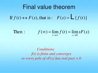
Final value theorem Conditions: f(t) is finite and converges or every pole of sF(s) has real part < 0
Input Output System • If the input x(t)=δ (t), the output is called the impulse response. • If the input x(t)=u(t), the output is called the step response. • If the input x(t)=Asin(wt), and H(s) is stable, output steady state is A|H(jw)|sin(wt+H(jw)) • Poles: values of s at which TF infinity • Zeros: values of s at which TF = 0 • Matlab commands: bode, nyquist, Input d(t),u(t) Output y(t) H(s)
Input Output Stability • System is BIBO stable if any bounded input generates bounded output • Simple TF criteria: • After common factor cancellation • All poles have strictly negative real parts • Sufficient condition: • Asymptotically stable implies BIBO stable • Time domain criteria:
Example G1 is not BIBO stable G2 and G3 are
Stability in State Space • Internal stability refers to the behavior of state variables in x(t): are they always bounded, or do they all converge to zero as t ∞? • Input output stability is concerned about the variables in y, in relation to u.
Asymptotically Stable A system is asymptotically stable if for any arbitrary initial conditions, all variables in the system converge to 0 as t→∞ when input=0. All variables include y & its derivatives all state variables but y=Cx+Du=Cx if x→0 then y→0 only need to check x→0 0
Marginally Stable and unstable A system is marginally stable if it is not asymptotically stable but no variable ever diverge to infinity as t→∞, when input=0. Note: • At least one variable does not converge to 0, since system is not A.S. • At least one variable becomes constant, sustains everlasting oscillation • At least one eigen value on the jw axis A system is unstable if not A.S. nor M.S.
Thm: If a system is A.S. then it is BIBO-stable But BIBO-stable does not imply A.S. (mathematically)
If there is no pole/zero cancellation, BIBO-stable iff A.S. Exact pole/zero cancellation only happens mathematically, not in real systems. From now on, assume no p/z cancellation and hence: BIBO stable iff A.S. iff all char. val<0, iff all poles<0 iff all eigenvalues<0
A polynomial is said to be Hurwitz or stable if all of its roots are in O.L.H.P A system is stable if its char. polynomial is Hurwitz A nxn matrix is called Hurwitz or stable if its char. poly det(sI-A) is Hurwitz, or if all eigenvalues have real parts<0
Routh-Hurwitz Method From now on, when we say stability we mean A.S. / M.S. or unstable. We assume no pole/zero cancellation, A.S. BIBO stable M.S./unstable not BIBO stable Since stability is determined by denominator, so just work with d(s)
Repeat the process until s0 row Stability criterion: • d(s) is A.S. iff 1st col have same sign • the # of sign changes in 1st col = # of roots in right half plane Note: if highest coeff in d(s) is 1, A.S. 1st col >0 If all roots of d(s) are <0, d(s) is Hurwitz
Example: ←has roots:3,2,-1
(1x3-2x5)/1=-7 (1x10-2x0)/1=10 (-7x5-1x10)/-7
Routh Criteria Regular case: (1) A.S. 1st col. all same sign (2)#sign changes in 1st col. =#roots with Re(.)>0 Special case 1: one whole row=0 Solution: 1) use prev. row to form aux. eq. A(s)=0 2) get 3) use coeff of in 0-row 4) continue
Example ←whole row=0
Useful case: parameter in d(s) How to use: 1) form table as usual 2) set 1st col. >0 3) solve for parameter range for A.S. 2’) set one in 1st col=0 3’) solve for parameter that leads to M.S. or leads to sustained oscillation
Example + s+3 s(s+2)(s+1) Kp