Constructing MDS Representations
Constructing MDS Representations. 김찬주 2010-01-12. Constructing MDS Representations Constructing Ratio MDS Solutions Constructing Ordinal MDS Solutions Comparing Ordinal and Ratio MDS Solutions On Flat and Curved Geometries General Properties of Distance Representations.


Constructing MDS Representations
E N D
Presentation Transcript
Constructing MDS Representations 김찬주 2010-01-12
Constructing MDS Representations • Constructing Ratio MDS Solutions • Constructing Ordinal MDS Solutions • Comparing Ordinal and Ratio MDS Solutions • On Flat and Curved Geometries • General Properties of Distance Representations • Construct MDS representations by hand. • Discuss constructions in some detail for ratio MDS and for ordinal MDS • Geometries.
1. Constructing Ratio MDS solutions • Ratio MDS • Represent the data such that their ratios would correspond to the ratios of the distances in the MDS space.
A Ruler-and-Compass Approach to Ratio MDS • Identify cities that are farthest from each other and choose a scale factor s. • Elaborate our two-point configuration by picking one of the remaining cities
A Ruler-and-Compass Approach to Ratio MDS • Continue by adding further points, then Figure 2.4 • Distances of points correspond to the distances in Table 2.1, except for an overall scale factor s.
A Ruler-and-Compass Approach to Ratio MDS • Replace the numbers with city names, then Figure 2.5. • Reflect the map along the horizontal direction, the Figure 2.6
A Ruler-and-Compass Approach to Ratio MDS • Rotate the map somewhat in a clockwise direction, then Figure 2.7
Admissible Transformations of Ratio MDS Configuration • Transformation often make MDS representations easier to look at. • Admissibletransformation • do not change the relations among the MDS distances. • rigid motions, dilations • Inadmissibletransformation • destroy the relationship between MDS distances.
Admissible Transformations of Ratio MDS Configuration • Rigid motion = isometry • The metric properties of the configuration, that is, distances between its points.
2. Constructing Ordinal MDS Solutions • Ordinal MDS • Only requires the order of the data • When only greater than and equal relations are considered informative.
A Ruler-and-Compass Approach to Ordinal MDS • Pick a pair of cities that define the first two points of the configuration. • If the cities 2 and 3 are picked as before, then Figure 2.1
A Ruler-and-Compass Approach to Ordinal MDS • Add point 9 to this configuration • d39: 36, d29 : 41 • d39< d29 • Solution set or solution space for the placing point 9. • Each point if this region could be chosen as point 9.
A Ruler-and-Compass Approach to Ordinal MDS • d23: 45 • d29< d23 • d39 < d23
A Ruler-and-Compass Approach to Ordinal MDS • Superimposing Figures 2.9 and 2.10 • d39 < d29 • d29 < d23 • d39 < d23 • Comparing Figure 2.2, Figure 2.11 is much more indeterminate. • Ordinal MDS • The reason for this increased indeterminacy lies in the weaker constraints. • only the order of the data determines the distances in MDS space.
A Ruler-and-Compass Approach to Ordinal MDS • Arbitrarily select one point from the solution set to represent object 9. • Add point 5. • (a) d25 < d29 • (b) d35 < d39 • (c) d59 < d53 • (d) d59 < d25 • (e) d35 < d25 • Point 5 must be placed that it satisfies all inequality conditions, (a) through (e).
Solution Spaces in Ordinal MDS • It may happen that the solution space is empty. • In Figure 2.11, assume that we had picked point 9’’. • Then add a point 10 to the configuration {2, 3, 9’’}. • The solution space for point 10 is empty. Figure 2.13
Solution Spaces in Ordinal MDS • Solution space for each newly added point shrinks in size at a rapidly accelerating rate. • The number of inequalities that determine the solution spaces grows mush faster than the number of points in the configuration. • Generally, with n points, • we obtain n·n = n2distancesdij • n2 – ndistancesexcept all dii • (n2 – n )/2 = (n) ( n – 1 )/2 relevant distances • All of these distances can be compared among each other • n = 4 16 inequalities, n = 50 749,700 inequalities
Isotonic Transformations • Isotonic transformation • play the same role in ordinal MDS as similarity transformations in ratio MDS. • comprise all transformations of a point configuration that leave the order relations of the distances unchanged (invariant). • include the isometric transformations. • An ordinal MDS solution is determined up to isotonic transformations because as long as the order of the distances is not changed, any configuration is as good an ordinal MDS representation as any other.
3. Comparing Ordinal and Ratio MDS Solutions • Treating the date as ordinal information only may be sufficient for reconstructing the original map. • Order relations in a data matrix like Table 2.3 are on pairs of pairs of objects, not just on pairs of objects. • We would have weak information, and in the first, obviously not. • Ratio and ordinal MDS solutions are almost always very similar in practice.
3. Comparing Ordinal and Ratio MDS Solutions • Why do ordinal MDS at all? • The answer typically relates to scale level considerations on the data. • Ex) A subject is given a 9-point on the data. • 1 = very poor, to 9 = very good. • The subject judges three pictures (A, B, and C) on this scale and arrives at the judgments A=8, B=7, C=1.
4. On Flat and Curved Geometries • In Figure 2.8, Stockholm has about the same Y-coordinate as points in Scotland. Geographically, however, Stockholm lies farther to the north than Scotland. • These distances were measured on a map printed on the pages of an atlas, and not measured over the curved surface of the globe. • Any geographical map that is flat is wrong in one way or another.
4. On Flat and Curved Geometries • The usual method projects the globe’s surface by rays emanating from the globe’s center onto the surface of a cylinder that encompasses the globe and touches it on the Equator. • Although the map is quite accurate for small areas, the size of the polar regions is greatly exaggerated.
4. On Flat and Curved Geometries • Euclidean geometry is flatand naturalgeometry. • The surface of the globe is a curved geometry. • Measure distance • Sum of the angles in a triangle • MDS almost always is carried out in Euclidean geometry.
5. General Properties of Distance Representations • A geometry that allows one to measure the distances between its points is called a metric geometry. • Properties • nonnegativity dii= djj = 0 ≤ dij • symmetry dij = dji • triangle inequality dij ≤ dik + dkj • Ex) Trivial distance defined by dij = 1 (if i ≠ j) and dij= 0 (if i = j)
5. General Properties of Distance Representations • Proximities where pij= pjidoes not hold for all i and j. • typical for the social relation “linking” between person. • Can not be represented directly in any metric geometry. • Symmetry is always a precondition for MDS. • The other properties of distances may or may not be necessary conditions for MDS. When piis are not equal or if any pii is greater than any pij (i ≠ j). • In ordinal MDS: no problem • In ratio MDS: serious problem